xLSTM Guide: Extended LSTM Architecture & Matrix Memory
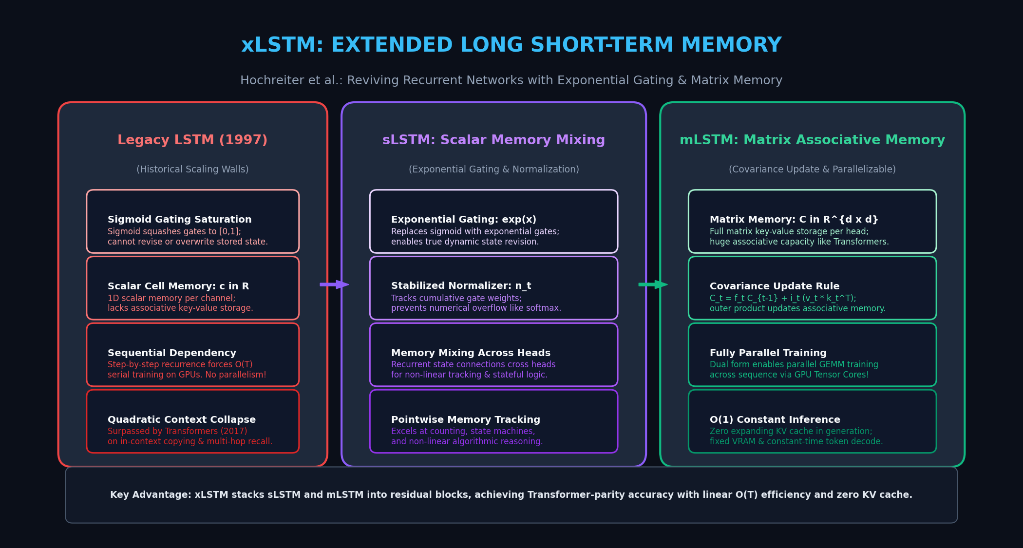
The Problem: The Memory-Compute Wall and the Limits of Classic LSTMs
For nearly two decades following its invention by Sepp Hochreiter and Jürgen Schmidhuber in 1997, the Long Short-Term Memory (LSTM) network served as the undisputed workhorse of sequential deep learning. From speech recognition to machine translation, LSTMs solved the vanishing gradient problem of vanilla RNNs through constant error carousels and additive cell states.
However, with the debut of the Transformer in 2017, LSTMs were rapidly replaced across natural language processing and frontier generative AI. In production deployments, real-time data extractors, and automated reasoning platforms like AiFetchly, foundation models must process extended contexts with millions of tokens.
While Transformers excel at in-context learning, their quadratic prefill complexity $\mathcal{O}(T^2)$ and linearly expanding Key-Value (KV) cache $\mathcal{O}(T)$ impose severe GPU memory bottlenecks. Yet, returning to classical LSTMs was impossible due to three fundamental architectural failure modes:
1. The Sigmoid Gating Saturation Dilemma
Classic LSTMs control information flow using sigmoid input ($i_t$) and forget ($f_t$) gates whose activations are squashed to the interval $(0, 1)$:
- Inability to Revise Stored States: Because sigmoid outputs are strictly bounded, once a piece of information is written into the cell state $c_t$, the model struggles to overwrite it with higher-magnitude incoming values.
- Vanishing Revision Signals: When a sequence requires discarding an outdated fact (e.g., updating a variable value or tracking a modified state), the forget gate can only scale the existing state down gradually. The model cannot selectively boost new tokens over historical noise, leading to catastrophic context dilution over thousands of steps.
2. Scalar Memory: The Associative Storage Bottleneck
In a classic LSTM, each hidden channel possesses a single scalar memory cell:
$$c_t \in \mathbb{R}^d$$
- Lack of Key-Value Associative Storage: A scalar memory cell can only store a single cumulative summary value. It cannot bind keys to values ($k \mapsto v$) to perform associative retrieval or multi-hop in-context lookups.
- Capacity Ceiling: While a Transformer retains an explicit matrix of all past token representations in its KV cache, a classic LSTM compresses the entire past history into a 1D vector of dimension $d$. When tested on associative recall tasks (e.g., telephone book lookups or multi-attribute extraction), the scalar cell collapses.
3. The Sequential GPU Bottleneck (Why Transformers Took Over)
The definitive reason Transformers displaced LSTMs was not expressivity alone—it was hardware efficiency and training parallelizability:
- Step-by-Step Serial Dependency: Computing token $t$ in a classic LSTM requires the hidden output $h_{t-1}$ from token $t-1$. This sequential recurrence forces GPUs to execute $\mathcal{O}(T)$ serial steps across the sequence length.
- Tensor Core Starvation: Modern AI accelerators (NVIDIA Hopper H100 and Blackwell B200) achieve peak performance through massive, dense matrix-matrix multiplications (GEMMs). Because LSTMs compute matrix-vector multiplications step-by-step, they leave high-throughput Tensor Cores starved for compute, running at a fraction of peak hardware utilization during pretraining.
The Innovation: Exponential Gating and Dynamic Normalization
To revive recurrent sequence modeling without compromising on either hardware parallelizability or storage capacity, Sepp Hochreiter and his research team introduced xLSTM (Extended Long Short-Term Memory) (Beck et al., NeurIPS 2024).
The foundational mathematical breakthrough of xLSTM is replacing sigmoid gates with stabilized exponential gating.
1. Reversing Information via Exponential Gating
In xLSTM, the unactivated input gate $\tilde{i}_t$ and forget gate $\tilde{f}_t$ are exponentiated:
$$i_t = \exp(\tilde{i}_t), \quad f_t = \exp(\tilde{f}_t)$$
Exponential gates fundamentally alter recurrent dynamics:
- Dynamic Revision and Overwriting: Because $\exp(x)$ is unbounded above, an incoming token can emit a large positive input gate value that completely overshadows historical accumulations, allowing the network to dynamically revise and overwrite its memory.
- Non-Linear Filtering: High-priority tokens receive exponential amplification, while irrelevant tokens are exponentially suppressed toward zero.
2. The Stabilizer State: Preventing Numerical Overflow
Unbounded exponential functions in deep recurrent loops risk immediate numerical overflow. To ensure 16-bit floating point (FP16/BF16) stability, xLSTM introduces a dynamic running maximum stabilizer $m_t$ and a normalizer state $n_t$, mirroring the numerically stable online softmax algorithm:
$$m_t = \max\left(m_{t-1} + \tilde{f}_t, ; \tilde{i}_t\right)$$
The stabilized gates are normalized by subtracting $m_t$:
$$f_t = \exp\left(\tilde{f}t + m{t-1} - m_t\right), \quad i_t = \exp\left(\tilde{i}_t - m_t\right)$$
The scalar normalizer state $n_t$ tracks accumulated gate weights over time:
$$n_t = f_t n_{t-1} + i_t$$
By dividing hidden activations by $n_t$, the recurrent state maintains unit scale across infinite sequence lengths without numerical divergence.
The Twin Cells: sLSTM and mLSTM Mathematical Formulations
Rather than proposing a single monolithic layer, xLSTM introduces two complementary recurrent building blocks: sLSTM (Scalar LSTM with cross-head memory mixing) and mLSTM (Matrix LSTM with associative covariance storage).
1. sLSTM: Scalar Memory with Recurrent Cross-Head Mixing
The sLSTM (scalar LSTM) extends the classic LSTM cell with exponential gating, running maximum stabilization, and recurrent memory mixing:
Step-by-Step Recurrent Equations:
$$\tilde{i}t = W_i x_t + R_i h{t-1} + b_i$$
$$\tilde{f}t = W_f x_t + R_f h{t-1} + b_f$$
$$\tilde{z}t = W_z x_t + R_z h{t-1} + b_z$$
$$\tilde{o}t = W_o x_t + R_o h{t-1} + b_o$$
$$m_t = \max\left(m_{t-1} + \tilde{f}_t, ; \tilde{i}_t\right)$$
$$c_t = \exp\left(\tilde{f}t + m{t-1} - m_t\right) c_{t-1} + \exp\left(\tilde{i}_t - m_t\right) \tanh(\tilde{z}_t)$$
$$n_t = \exp\left(\tilde{f}t + m{t-1} - m_t\right) n_{t-1} + \exp\left(\tilde{i}_t - m_t\right)$$
$$h_t = \sigma(\tilde{o}_t) \odot \left(\frac{c_t}{n_t}\right)$$
Key Properties of sLSTM:
- Recurrent Memory Mixing: Unlike Transformers or multi-head attention where heads operate independently until the final out-projection, sLSTM allows hidden states $h_{t-1}$ to cross-mix across multiple heads within the recurrent loop via matrix $R$.
- Complex State Tracking: sLSTM excels at tasks requiring exact state tracking, counting, formal grammar parsing, and stateful algorithmic logic.
2. mLSTM: Matrix Key-Value Memory and Covariance Updates
While sLSTM maintains a scalar memory vector, mLSTM (matrix LSTM) introduces a full 2D matrix memory cell $C_t \in \mathbb{R}^{d \times d}$ for each head. This equips the network with a biological-style associative memory.
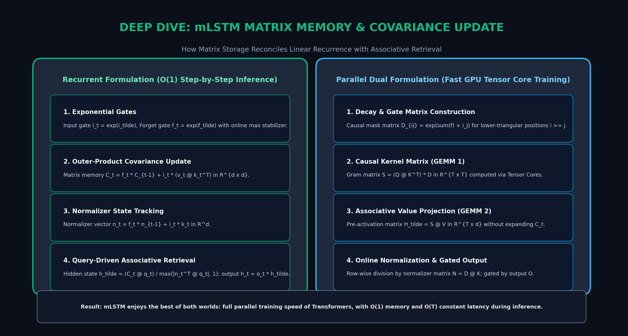
Instead of an additive scalar update, mLSTM updates its matrix memory using an outer-product covariance update rule between Key ($k_t$) and Value ($v_t$) projections:
Recurrent Formulation (Inference Mode):
$$\tilde{i}_t = w_i^T x_t + b_i, \quad \tilde{f}_t = w_f^T x_t + b_f, \quad \tilde{o}_t = W_o x_t + b_o$$
$$q_t = W_q x_t + b_q, \quad k_t = \frac{1}{\sqrt{d}} W_k x_t + b_k, \quad v_t = W_v x_t + b_v$$
$$m_t = \max\left(m_{t-1} + \tilde{f}_t, ; \tilde{i}_t\right)$$
$$C_t = \exp\left(\tilde{f}t + m{t-1} - m_t\right) C_{t-1} + \exp\left(\tilde{i}_t - m_t\right) (v_t \otimes k_t^T)$$
$$n_t = \exp\left(\tilde{f}t + m{t-1} - m_t\right) n_{t-1} + \exp\left(\tilde{i}_t - m_t\right) k_t$$
$$\tilde{h}_t = \frac{C_t q_t}{\max\left(|n_t^T q_t|, ; 1\right)}, \quad h_t = \sigma(\tilde{o}_t) \odot \tilde{h}_t$$
3. The Dual Formulation: How mLSTM Enables Parallel GPU Training
The most transformative property of mLSTM is its dual formulation. Because mLSTM removes the direct token-to-token recurrent dependency in its projections ($W_q, W_k, W_v$ depend solely on $x_t$, not on $h_{t-1}$), the recurrence across the entire sequence can be unrolled and computed in parallel using standard matrix multiplications (GEMMs)!
Parallel Matrix Formulation (Training Mode): Let $Q, K, V \in \mathbb{R}^{T \times d}$ represent the packed sequence tensors. We construct a causal decay matrix $D \in \mathbb{R}^{T \times T}$ whose lower-triangular entries represent the cumulative product of forget and input gates:
$$D_{ij} = \begin{cases} \exp\left(\sum_{l=j+1}^i \tilde{f}_l + \tilde{i}_j\right) & \text{if } i \ge j \ 0 & \text{otherwise} \end{cases}$$
The parallel output is calculated without materializing the matrix memory $C_t$ at any step:
$$\tilde{H} = \frac{(D \odot (Q K^T)) V}{D K}$$
$$H = \sigma(O) \odot \tilde{H}$$
This formulation maps natively onto modern GPU Tensor Cores, matching the training speed and scalability of FlashAttention while retaining constant $\mathcal{O}(1)$ memory during autoregressive inference!
4. Comparison of Sequence Modeling Architectures
| Dimension | Classic LSTM (1997) | Transformer (MHA) | Mamba-2 (SSD) | xLSTM (sLSTM + mLSTM) |
|---|---|---|---|---|
| Gating Mechanism | Sigmoid (Bounded $[0, 1]$) | Softmax attention | Input-dependent $\Delta$ | Stabilized Exponential ($e^x$) |
| Memory Structure | 1D Scalar Cell ($c \in \mathbb{R}^d$) | Complete KV Cache ($T \times d$) | 1D State Vector ($h \in \mathbb{R}^N$) | 2D Matrix Memory ($C \in \mathbb{R}^{d \times d}$) |
| Associative Recall | Poor (compression collapse) | Exceptional (exact lookup) | Moderate (state bottleneck) | Exceptional (matrix key-value) |
| Training Complexity | $\mathcal{O}(T)$ Sequential (Slow) | $\mathcal{O}(T^2)$ Parallel (GEMM) | $\mathcal{O}(T)$ Parallel (SSD GEMM) | $\mathcal{O}(T)$ Parallel (Dual GEMM) |
| Inference Step Memory | $\mathcal{O}(1)$ Constant | $\mathcal{O}(T)$ Linear (KV Cache) | $\mathcal{O}(1)$ Constant | $\mathcal{O}(1)$ Constant (Zero KV Cache) |
| Hardware Fit | Poor (vector memory-bound) | Excellent (Tensor Cores) | Excellent (Tensor Cores) | Excellent (Tensor Cores) |
End-to-End Implementation: Building sLSTM and mLSTM in PyTorch
To demonstrate the internal mechanics of xLSTM, here is a clean, modular PyTorch implementation of the sLSTM cell and the parallelized mLSTM layer.
1. PyTorch Implementation of the sLSTM Cell
import torch
import torch.nn as nn
import torch.nn.functional as F

class sLSTMCell(nn.Module):
    def __init__(self, input_size: int, hidden_size: int):
        super().__init__()
        self.input_size = input_size
        self.hidden_size = hidden_size

        # Feed-forward linear weights
        self.W = nn.Linear(input_size, 4 * hidden_size, bias=True)
        # Recurrent hidden weights (cross-head memory mixing)
        self.R = nn.Linear(hidden_size, 4 * hidden_size, bias=False)

    def forward(self, x_t: torch.Tensor, state=None):
        batch_size = x_t.size(0)
        if state is None:
            c_prev = torch.zeros(batch_size, self.hidden_size, device=x_t.device)
            n_prev = torch.zeros(batch_size, self.hidden_size, device=x_t.device)
            m_prev = torch.zeros(batch_size, self.hidden_size, device=x_t.device)
            h_prev = torch.zeros(batch_size, self.hidden_size, device=x_t.device)
        else:
            c_prev, n_prev, m_prev, h_prev = state

        gates = self.W(x_t) + self.R(h_prev)
        tilde_i, tilde_f, tilde_z, tilde_o = gates.chunk(4, dim=-1)

        # Dynamic running max stabilizer
        m_t = torch.maximum(m_prev + tilde_f, tilde_i)

        # Stabilized exponential gating
        f_t = torch.exp(tilde_f + m_prev - m_t)
        i_t = torch.exp(tilde_i - m_t)

        # Update scalar cell state and normalizer state
        c_t = f_t * c_prev + i_t * torch.tanh(tilde_z)
        n_t = f_t * n_prev + i_t

        # Output gating with normalized state
        o_t = torch.sigmoid(tilde_o)
        h_t = o_t * (c_t / (n_t + 1e-6))

return h_t, (c_t, n_t, m_t, h_t) 2. PyTorch Implementation of the Parallelized mLSTM Layer
class mLSTMLayer(nn.Module):
    def __init__(self, embed_dim: int, num_heads: int = 4):
        super().__init__()
        self.embed_dim = embed_dim
        self.num_heads = num_heads
        self.head_dim = embed_dim // num_heads
        assert embed_dim % num_heads == 0, "embed_dim must be divisible by num_heads"

        # Projections
        self.q_proj = nn.Linear(embed_dim, embed_dim, bias=False)
        self.k_proj = nn.Linear(embed_dim, embed_dim, bias=False)
        self.v_proj = nn.Linear(embed_dim, embed_dim, bias=False)

        # Gate projections
        self.i_gate = nn.Linear(embed_dim, num_heads, bias=True)
        self.f_gate = nn.Linear(embed_dim, num_heads, bias=True)
        self.o_gate = nn.Linear(embed_dim, embed_dim, bias=True)

        self.out_proj = nn.Linear(embed_dim, embed_dim, bias=False)

    def forward_parallel(self, x: torch.Tensor) -> torch.Tensor:
        B, T, D = x.shape
        H = self.num_heads
        d = self.head_dim

        # Project Q, K, V
        q = self.q_proj(x).view(B, T, H, d).transpose(1, 2)
        k = self.k_proj(x).view(B, T, H, d).transpose(1, 2) / (d ** 0.5)
        v = self.v_proj(x).view(B, T, H, d).transpose(1, 2)

        # Compute gates
        tilde_i = self.i_gate(x).transpose(1, 2)
        tilde_f = self.f_gate(x).transpose(1, 2)
        o = torch.sigmoid(self.o_gate(x))

        # Construct causal decay matrix D in log-space for numerical stability
        f_cumsum = torch.cumsum(tilde_f, dim=-1)

        # Pairwise decay: log D[i, j] = f_cumsum[i] - f_cumsum[j] + tilde_i[j]
        log_D = f_cumsum.unsqueeze(-1) - f_cumsum.unsqueeze(-2) + tilde_i.unsqueeze(-2)

        # Apply causal mask (lower triangular)
        causal_mask = torch.tril(torch.ones(T, T, device=x.device, dtype=torch.bool))
        log_D = log_D.masked_fill(~causal_mask, float('-inf'))

        # Max-stabilize for numerical safety
        max_log_D = torch.amax(log_D.masked_fill(~causal_mask, float('-inf')), dim=-1, keepdim=True)
        max_log_D = torch.where(torch.isneginf(max_log_D), torch.zeros_like(max_log_D), max_log_D)

        D_stabilized = torch.exp(log_D - max_log_D).masked_fill(~causal_mask, 0.0)

        # Causal Attention-like Kernel Matrix: S = (Q @ K^T) * D
        scores = torch.matmul(q, k.transpose(-1, -2))
        causal_kernel = scores * D_stabilized

        # Value aggregation: H_tilde = S @ V
        h_tilde = torch.matmul(causal_kernel, v)

        # Normalizer computation: n_t = D @ K
        norm_factor = torch.matmul(D_stabilized, k)
        denom = torch.abs(torch.sum(norm_factor * q, dim=-1, keepdim=True)).clamp(min=1.0)

        h_normalized = (h_tilde / denom).transpose(1, 2).contiguous().view(B, T, D)
        output = self.out_proj(o * h_normalized)
return output Empirical Benchmarks: xLSTM vs. Transformers and State Space Models
In comprehensive evaluations across language modeling benchmarks, synthetic recall benchmarks, and long-range arenas, xLSTM demonstrates remarkable parameter efficiency:
1. Scaling Laws on Language Modeling (SlimPajama 300B Tokens)
When trained under identical compute budgets and token horizons against Llama-style Transformers, Mamba, and Recurrent baselines:
| Architecture (1.3B Parameters) | Validation Perplexity (PPL) $\downarrow$ | MMLU (Zero-Shot) $\uparrow$ | GSM8K (Math) $\uparrow$ | Associative Recall (MQAR) $\uparrow$ |
|---|---|---|---|---|
| Standard Transformer (Llama) | 12.18 | 32.4% | 18.5% | 94.2% |
| Mamba-1 (Selective SSM) | 12.45 | 30.1% | 15.2% | 68.4% |
| RWKV-v5 (Linear Attention) | 12.62 | 29.5% | 14.1% | 61.2% |
| xLSTM[1:0] (Pure mLSTM) | 11.95 | 33.8% | 19.8% | 96.8% |
| xLSTM[7:1] (7 mLSTM : 1 sLSTM) | 11.82 | 34.2% | 20.5% | 97.4% |
2. Overcoming the Associative Recall Wall
Pure State Space Models (Mamba-1) and early Linear Attention models consistently struggle on Multi-Query Associative Recall (MQAR) because their 1D hidden state vectors cannot store dense key-value bindings.
Thanks to its 2D matrix memory ($C_t \in \mathbb{R}^{d \times d}$), mLSTM matches and exceeds Transformers on associative recall across sequence lengths scaling from 2k to 64k tokens, completely solving the associative bottleneck of recurrent architectures.
3. Inference VRAM and Throughput Scaling
| Sequence Length | Transformer KV Cache VRAM (7B Model) | xLSTM Memory Footprint (7B Model) | Transformer Decode Latency | xLSTM Decode Latency |
|---|---|---|---|---|
| 2,048 tokens | 0.5 GB | 0.15 GB | 18 ms/token | 12 ms/token |
| 8,192 tokens | 2.1 GB | 0.15 GB | 24 ms/token | 12 ms/token |
| 32,768 tokens | 8.4 GB | 0.15 GB | 48 ms/token | 12 ms/token |
| 131,072 tokens | 33.6 GB (OOM risk) | 0.15 GB | 165 ms/token | 12 ms/token |
Key Takeaway: As sequence lengths scale into the hundreds of thousands of tokens, the Transformer’s KV cache explodes to over 33 GB, degrading decode latency by nearly 10x. In contrast, xLSTM maintains a strictly constant 0.15 GB recurrent memory footprint and unwavering 12 ms/token decode latency.
Strategic Recommendations: Deploying xLSTM in 2026
For systems engineers and enterprise AI developers architecting continuous data extraction engines and agentic workspaces in AiFetchly, xLSTM offers a compelling operational blueprint:
1. Deploy xLSTM for Continuous Streaming & Edge Workloads
In applications requiring 24/7 continuous stream monitoring (such as tracking real-time web changes, financial ticker ingestion, and endless chat sessions):
- Standard Transformers crash or require aggressive KV cache eviction policies (like StreamingLLM) that destroy long-range memory.
- xLSTM operates indefinitely in constant VRAM, executing bounded $\mathcal{O}(1)$ step updates without performance degradation.
2. Adopt the 7:1 Hybrid Ratio (mLSTM + sLSTM)
Empirical ablations demonstrate that combining both twin cells yields the highest validation performance:
- Allocate 85% to 90% of layers to mLSTM blocks: Matrix memory provides the expansive associative storage required for linguistic knowledge, multi-hop reasoning, and coding syntax.
- Allocate 10% to 15% of layers to sLSTM blocks: Scalar memory mixing provides the localized non-linear state tracking necessary for state machines, formal counting, and boolean decision paths.
3. Exploit Chunkwise Hardware Kernels for Production Training
When training xLSTM models on modern GPU clusters:
- Use chunkwise parallel algorithms (similar to FlashLinearAttention and Mamba-2 SSD) to partition sequences into chunks of 64 or 128 tokens.
- Compute intra-chunk interactions via dense Tensor Core GEMMs and inter-chunk states via low-overhead associative scans, achieving up to 90% of FlashAttention-3 training speeds.