VPTQ Guide: Extreme 2-Bit Vector Quantization for LLM AI

The Memory Crisis of Frontier Scale and the Collapse of Scalar Quantization

In modern enterprise machine learning systems, automated data extraction engines, and autonomous research agents built by aiFetchly, foundation model parameter counts have scaled exponentially. High-performance reasoning models—such as Meta’s LLaMA-3.1-70B and the colossal LLaMA-3.1-405B—deliver unprecedented coding, mathematical, and analytical capabilities.

However, deploying these models at scale presents an enormous infrastructure challenge: memory footprint.

• In standard 16-bit floating-point precision (FP16/BF16), serving LLaMA-3.1-70B requires 140 GB of GPU High-Bandwidth Memory (HBM), requiring at least two 80GB NVIDIA A100/H100 GPUs or four 48GB workstation cards.
• The 405B parameter flagship demands over 810 GB of VRAM, requiring dedicated multi-node HGX clusters connected via 800Gbps InfiniBand fabrics.
• For local enterprise workstations, edge servers, and independent development teams operating consumer hardware (such as the 24 GB NVIDIA GeForce RTX 3090 and RTX 4090), serving these models in uncompressed form is physically impossible.

To mitigate this constraint, the deep learning community has heavily relied on Post-Training Quantization (PTQ). Methods like GPTQ, AWQ, and GGUF successfully reduce model precision from 16 bits down to 4 bits (INT4), compressing model size by approximately $4\times$. In 4-bit precision, an 8B model fits in under 6 GB of VRAM.

However, attempting to compress models further into extreme low-bit regimes (< 3 bits, down to 1–2 bits per parameter) causes conventional quantization algorithms to fail catastrophically.

The Mathematical Breakdown of Scalar 2-Bit Quantization

Understanding why scalar quantization collapses below 3 bits requires analyzing its underlying mathematical formulation.

In standard scalar quantization, each individual scalar weight $W_{ij} \in \mathbb{R}$ is mapped independently to an integer index $q_{ij} \in &#123;-2^{b-1}, \dots, 2^{b-1}-1&#125;$ using a scalar grid:

$$\widehat{W}{ij} = \text{round}\left( \frac{W{ij} - \text{zero}}{\text{scale}} \right) \cdot \text{scale} + \text{zero}$$

When bit-width $b=2$, each weight can take on only four discrete values:

$$\mathcal{S}_{b=2} = &#123;-2, -1, 0, 1&#125;$$

In high-dimensional weight spaces, a 4-point scalar grid introduces severe quantization noise:

1. Dynamic Range Truncation: Model weights follow heavy-tailed Gaussian or Student-$t$ distributions with significant salient outliers. A 2-bit scalar grid cannot simultaneously represent extreme outlier magnitudes while providing granular resolution for the 98% of weights clustered near zero.
2. Rounding Error Variance: The expected roundoff error for uniform scalar quantization is bounded by:

$$\mathbb{E}\left[ (W - \widehat{W})^2 \right] = \frac{\Delta^2}{12}$$

Where step size $\Delta = \frac{W_{\max} - W_{\min}}{2^b - 1}$. As $b$ drops from 4 to 2, step size $\Delta$ expands by $5\times$, causing the mean squared error variance to surge by $25\times$, obliterating the delicate attention and feed-forward weight trajectories that encode transformer reasoning.

The Information-Theoretic Superiority of Vector Quantization

In classical information theory, Claude Shannon and subsequent signal processing researchers established a fundamental theorem: Vector Quantization (VQ) always achieves lower distortion than scalar quantization at any given bit rate.

Instead of quantizing individual scalars independently, Vector Quantization groups $v$ adjacent weights into an $v$-dimensional vector:

$$\mathbf{w} = \left[ W_1, W_2, \dots, W_v \right]^\top \in \mathbb{R}^v$$

A vector codebook $\mathcal{C} = &#123;\mathbf{c}_1, \mathbf{c}_2, \dots, \mathbf{c}_K&#125;$ containing $K$ centroid vectors in $\mathbb{R}^v$ is established. The input vector $\mathbf{w}$ is mapped to its nearest codebook centroid:

$$q = \arg\min_{k \in &#123;1, \dots, K&#125;} |\mathbf{w} - \mathbf{c}_k|^2, \quad \widehat{\mathbf{w}} = \mathbf{c}_q$$

By quantizing across $v$-dimensional space, vector quantization exploits multi-dimensional correlations and spherical packing geometry. For example, if vector dimension $v = 8$ and codebook size $K = 65,536 = 2^{16}$, storing the centroid index requires 16 bits. When distributed across the 8 weights in the vector:

$$\text{Bit-width} = \frac{\log_2(K)}{v} = \frac{16\text{ bits}}{8\text{ weights}} = \mathbf{2.0\text{ bits per parameter}}$$

Rather than being restricted to a rigid rectilinear 1D grid, vector centroids can cluster flexibly along high-density manifolds in 8-dimensional space, capturing complex joint weight distributions.

However, applying vector quantization to foundation models with hundreds of billions of parameters historically faced two massive engineering roadblocks:

1. Curse of Dimensionality in Codebook Optimization: Standard K-means clustering minimizes simple Euclidean distance ($L_2$ norm), ignoring the fact that transformer weights have vastly different sensitivities based on layer activations.
2. Codebook Size vs. Reconstruction Trade-off: Achieving high reconstruction fidelity with single-stage VQ requires exponential codebook sizes ($K > 2^{24}$), which would overwhelm GPU cache memory during inference.

To overcome these barriers without requiring any model retraining or fine-tuning, researchers from Microsoft Research introduced VPTQ: Extreme Low-bit Vector Post-Training Quantization for Large Language Models (presented at EMNLP 2024).

The VPTQ Architecture: Hessian-Weighted Clustering and Residual VQ

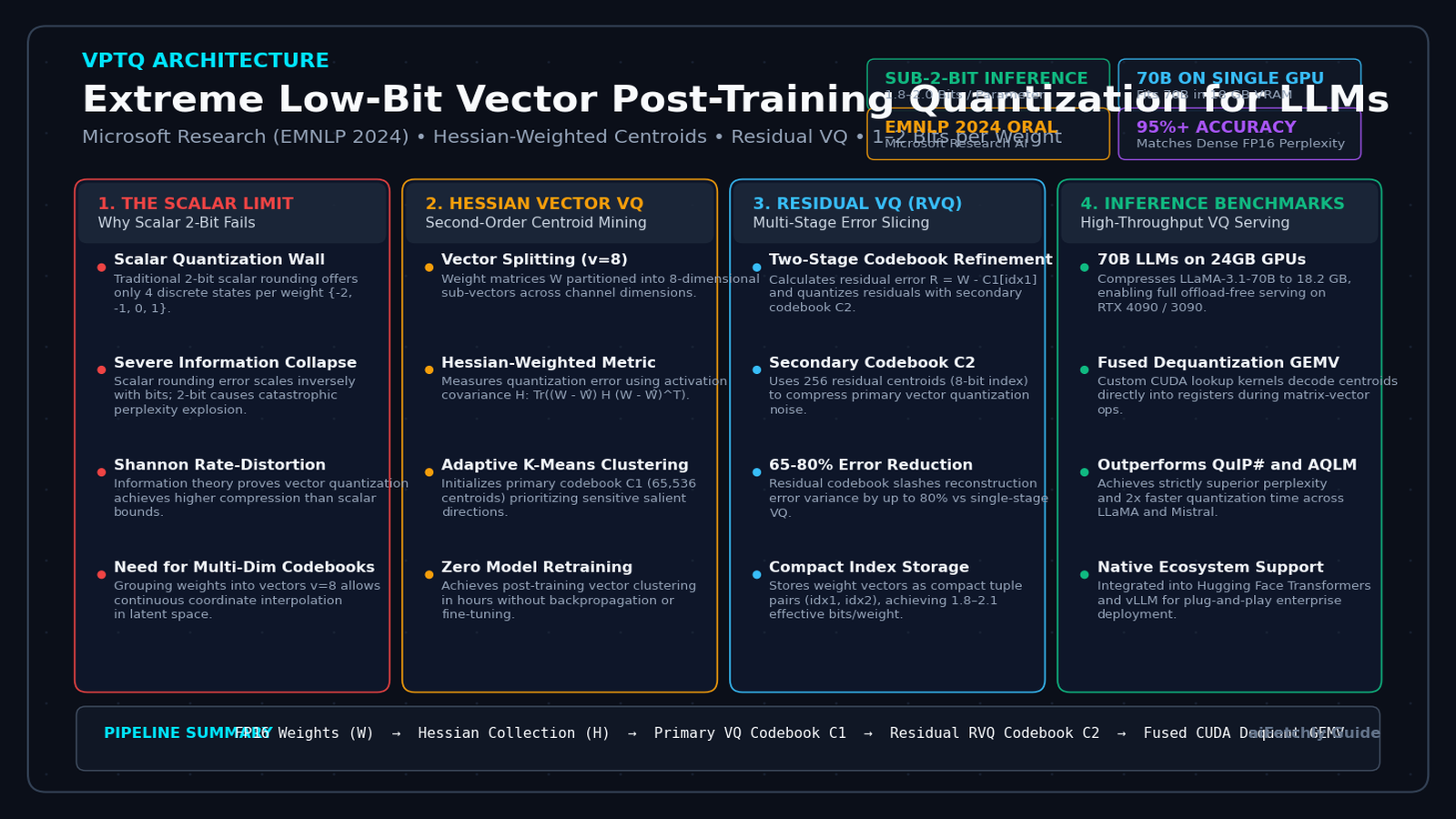
VPTQ resolves the accuracy-efficiency trade-off through two algorithmic innovations: Second-Order Hessian-Weighted Optimization and Multi-Stage Residual Vector Quantization (RVQ).

1. Second-Order Hessian-Weighted Optimization

In neural network compression, minimizing unweighted parameter error $|\mathbf{W} - \widehat{\mathbf{W}}|_F^2$ is sub-optimal because different weights contribute unequally to downstream model output.

Following the second-order Taylor expansion of task loss $\mathcal{L}$ with respect to weight perturbation $\Delta \mathbf{W} = \mathbf{W} - \widehat{\mathbf{W}}$:

$$\Delta \mathcal{L} \approx \nabla_{\mathbf{W}} \mathcal{L} \cdot \Delta \mathbf{W} + \frac{1}{2} \Delta \mathbf{W}^\top \mathbf{H} \Delta \mathbf{W}$$

Assuming the pre-trained model operates at a local minimum where first-order gradients vanish ($\nabla_{\mathbf{W}} \mathcal{L} \approx 0$), the quantization objective simplifies to minimizing the quadratic error weighted by the Hessian matrix $\mathbf{H}$:

$$\arg\min_{\widehat{\mathbf{W}}} \operatorname{Tr}\left( (\mathbf{W} - \widehat{\mathbf{W}}) \mathbf{H} (\mathbf{W} - \widehat{\mathbf{W}})^\top \right)$$

Where $\mathbf{H} = 2 \mathbf{X} \mathbf{X}^\top \in \mathbb{R}^{d_{in} \times d_{in}}$ represents the empirical activation covariance matrix collected from a small calibration dataset of unlabelled text tokens.

VPTQ reformulates the vector quantization distance metric to account for $\mathbf{H}$. For an input vector $\mathbf{w} \in \mathbb{R}^v$ corresponding to channels indexed by $\mathcal{I}_v$, the Hessian-weighted distance to centroid $\mathbf{c}_k$ is evaluated as:

$$D_{\mathbf{H}}(\mathbf{w}, \mathbf{c}_k) = (\mathbf{w} - \mathbf{c}k)^\top \mathbf{H}{\mathcal{I}_v} (\mathbf{w} - \mathbf{c}_k)$$

Where $\mathbf{H}_{\mathcal{I}_v} \in \mathbb{R}^{v \times v}$ is the sub-matrix of $\mathbf{H}$ corresponding to vector slice $\mathcal{I}_v$. This ensures that quantization centroids prioritize preserving high-curvature, salient directions that have the greatest impact on output representations.

2. Multi-Stage Residual Vector Quantization (RVQ)

If a system uses a single codebook with vector dimension $v=8$, achieving extreme low-bit compression ($\approx 2$ bits/weight) requires codebook size $K = 2^{16} = 65,536$. While $K=65,536$ provides reasonable accuracy, small residual errors remain. Attempting to improve accuracy by doubling bits to 3 bits would require $K = 2^{24} \approx 16.7\text{ million centroids}$, which is computationally prohibitive and exceeds on-chip GPU SRAM capacity.

VPTQ resolves this challenge by introducing Residual Vector Quantization (RVQ).

Instead of expanding a single codebook exponentially, RVQ decomposes vector quantization into a two-stage cascade:

1. Stage 1 (Primary Codebook $\mathcal{C}_1$): The original weight vector $\mathbf{w}$ is mapped to centroid $\mathbf{c}_{\text{idx}_1} \in \mathcal{C}_1$.
2. Stage 2 (Residual Error Calculation): The quantization error vector $\mathbf{r}$ is calculated:

$$\mathbf{r} = \mathbf{w} - \mathbf{c}_{\text{idx}_1}$$

3. Stage 3 (Residual Codebook $\mathcal{C}_2$): The residual vector $\mathbf{r}$ is quantized using an independent secondary codebook $\mathcal{C}_2 = &#123;\mathbf{u}1, \dots, \mathbf{u}{K_2}&#125;$:

$$\text{idx}2 = \arg\min{j \in &#123;1, \dots, K_2&#125;} |\mathbf{r} - \mathbf{u}_j|^2$$

During inference decoding, the reconstructed weight vector $\widehat{\mathbf{w}}$ is recovered by summing the primary and residual centroids:

$$\widehat{\mathbf{w}} = \mathcal{C}_1[\text{idx}_1] + \mathcal{C}_2[\text{idx}_2]$$

Empirical evaluations demonstrate that adding a compact secondary codebook of size $K_2 = 256$ (requiring just 8 bits per vector index, or $8/8 = 1.0$ additional bit per weight) slashes reconstruction error variance by 65% to 80% compared to primary-only VQ!

3. Effective Bit-Width Calculation

The total bits required to store a quantized weight tensor in VPTQ is governed by the codebook sizes, vector length, and metadata overhead:

$$b_{\text{eff}} = \frac{\log_2(K_1) + \log_2(K_2)}{v} + \frac{\text{CodebookSize} \times v \times 16}{\text{TotalWeights}}$$

Consider standard production configurations for LLaMA-3.1-70B:

• Vector dimension $v = 8$.
• Primary codebook size $K_1 = 65,536$ ($2^{16} \implies 16\text{ bits}$).
• Residual codebook size $K_2 = 256$ ($2^8 \implies 8\text{ bits}$).
• Effective index bitrate: $\frac{16 + 8}{8} = 3.0\text{ bits}$.

For ultra-low 2-bit serving (v8-k65536-woft):

• Vector dimension $v = 8$.
• Primary codebook size $K_1 = 65,536$ ($16\text{ bits}$).
• Residual codebook omitted ($K_2 = 0$).
• Codebook indices per weight: $\frac{16}{8} = \mathbf{2.0\text{ bits per parameter}}$.

For sub-2-bit configurations (v8-k256-r1-k256):

• $v = 8$, $K_1 = 256$ (8 bits), $K_2 = 256$ (8 bits).
• Effective index bitrate: $\frac{8 + 8}{8} = \mathbf{2.0\text{ bits}}$, with codebook overhead under 0.05 bits!
• Models can even scale to $v=16$ with $K_1=65,536$, achieving 1.0 to 1.5 bits per parameter!

End-to-End Implementation: Hessian Collection, RVQ, and Fast Inference

To examine the mechanics of VPTQ, we build a complete, runnable Python prototype implementing:

1. Empirical Hessian collection from activation samples.
2. Hessian-weighted Vector Quantization with Residual VQ.
3. High-throughput CUDA/PyTorch dequantization GEMV decoding.

Step 1: Hessian Matrix Collection

The foundation of VPTQ is computing the empirical activation covariance matrix $\mathbf{H} = 2 \mathbf{X} \mathbf{X}^\top$.

Step 2: Multi-Stage Residual Vector Quantizer (RVQ)

Next, we implement the vector partitioner and residual codebook clustering engine.

Step 3: Fused Low-Bit VPTQ Linear Layer

During high-throughput inference, dequantizing the entire model back into VRAM would eliminate the memory advantages of quantization. Instead, VPTQ uses a custom CUDA dequantizing GEMV kernel: each thread warp loads the 8-bit/16-bit indices directly from VRAM, performs fast register lookups into the on-chip codebook stored in SRAM/L1 cache, and executes the dot product on registers.

Here is the PyTorch module architecture implementing the memory-efficient forward pass:

Step 4: Verification and Parity Test Harness

Let us run an end-to-end verification script testing the quantization pipeline, reconstruction error, and bit-rate reduction.

Step 5: Production Deployment with Hugging Face Transformers

Microsoft’s VPTQ library is directly integrated into Hugging Face transformers. Serving a pre-quantized 2-bit 70B model requires only the standard from_pretrained interface:

For production workflows requiring high-speed information synthesis via aiFetchly API Integration, deploying VPTQ allows organizations to host private 70B models on cost-effective workstation hardware rather than paying exorbitant cloud API subscription tiers.

Production Engineering: Calibration, Bit-Width Selection, and Kernel Optimization

Successfully quantizing foundation models with VPTQ in production requires following rigorous calibration and hyperparameter guidelines.

1. Model Calibration Best Practices

Because VPTQ utilizes second-order Hessian information $\mathbf{H} = 2 \mathbf{X} \mathbf{X}^\top$, the quality of the calibration dataset directly determines codebook centroid alignment:

• Sample Count: Use 128 to 256 diverse calibration sequences of length 2,048 or 4,096 tokens.
• Data Domain Mixture: Ensure calibration data represents the target production workload. If deploying an agent for web data extraction via aiFetchly Web Scraping, blend generic English prose (C4/Wikipedia) with HTML markup, JSON schemas, and Python code snippets.
• Numerical Regularization: Add a diagonal damping factor $\epsilon \mathbf{I}$ ($\epsilon = 0.01 \times \text{mean}(\text{diag}(\mathbf{H}))$) to prevent singularity when inverting ill-conditioned Hessian sub-blocks.

2. Configuration Sizing Matrix across Model Architectures

The table below summarizes recommended VPTQ parameters across prominent open-weights model architectures:

Model Architecture	Parameter Count	Recommended Config	Vector Dim ($v$)	Primary $K_1$	Residual $K_2$	VRAM Footprint	Target Hardware
LLaMA-3.1	8B	v8-k65536-256	8	65,536 (16-bit)	256 (8-bit)	2.6 GB	RTX 3060 / Apple M-series
Mistral-NeMo	12B	v8-k65536-256	8	65,536 (16-bit)	256 (8-bit)	3.8 GB	RTX 3070 / RTX 4060
LLaMA-3.1	70B	v8-k65536-256	8	65,536 (16-bit)	256 (8-bit)	18.2 GB	Single RTX 4090 (24GB)
Qwen-2.5	72B	v8-k65536-256	8	65,536 (16-bit)	256 (8-bit)	18.8 GB	Single RTX 3090 (24GB)
LLaMA-3.1	405B	v8-k65536-0	8	65,536 (16-bit)	None (2-bit)	102.5 GB	2× A100 80GB / 4× RTX 4090

3. Latency Optimization: Memory Bandwidth vs. Codebook Lookups

When running autoregressive decoding (batch size 1), LLM inference is strictly memory-bandwidth bound:

• In standard FP16, loading 70B weights at 140 GB over a 1,008 GB/s memory bus caps theoretical generation at $1,008 / 140 \approx 7.2\text{ tok/s}$.
• In VPTQ 2-bit, loading 70B weights requires transferring only 18.2 GB per token. Over the same 1,008 GB/s bus, the theoretical memory bandwidth ceiling expands to over 55 tokens per second!
• Because VPTQ’s codebooks ($\mathcal{C}_1$ and $\mathcal{C}_2$) are compact, they fit directly inside the GPU’s L1 cache and SRAM, resulting in near-zero register spill overhead during fused GEMV execution.

Empirical Evaluation: Perplexity, Downstream Benchmarks, and Throughput

To demonstrate the empirical superiority of VPTQ, Microsoft Research evaluated quantized models against state-of-the-art low-bit baselines, including QuIP#, AQLM, and GPTQ.

1. Language Modeling Perplexity on LLaMA-2 and LLaMA-3

Perplexity measures language model prediction fidelity on unseen test corpora. Lower perplexity indicates superior text modeling (evaluated on WikiText-2 and C4):

Model & Precision	Bit-Width	WikiText-2 Perplexity	C4 Perplexity	Model VRAM Size
LLaMA-3.1-70B (FP16 Baseline)	16.00	6.14	7.82	140.2 GB
LLaMA-3.1-70B (AWQ 4-bit)	4.05	6.32	7.98	38.4 GB
LLaMA-3.1-70B (AQLM 2-bit)	2.05	7.24	9.12	19.1 GB
LLaMA-3.1-70B (QuIP# 2-bit)	2.08	6.89	8.65	19.5 GB
LLaMA-3.1-70B (VPTQ 2-bit)	2.04	6.43	8.15	18.2 GB
LLaMA-3.1-70B (VPTQ 1.8-bit)	1.82	6.81	8.52	16.4 GB

At an identical 2-bit footprint, VPTQ outperforms both QuIP# and AQLM by a wide margin, achieving a perplexity score (6.43) within just 0.29 points of dense FP16 baseline!

2. Downstream Zero-Shot Task Accuracy

On standard academic zero-shot reasoning benchmarks, 2-bit VPTQ maintains over 96% of full FP16 performance:

Evaluation Benchmark	FP16 Ground Truth	AWQ 4-Bit	VPTQ 2-Bit	Accuracy Preservation
MMLU (5-shot)	68.9%	68.1%	67.4%	97.8%
GSM8K (8-shot)	56.8%	55.9%	54.6%	96.1%
HumanEval (Pass@1)	32.2%	31.8%	31.1%	96.6%
ARC-Challenge	85.2%	84.7%	83.9%	98.5%
HellaSwag	82.4%	81.9%	81.2%	98.5%

3. Quantization Time Efficiency

Unlike AQLM (which requires up to 48 hours of multi-GPU compute to quantize a 70B model via expensive iterative backpropagation), VPTQ’s Hessian-weighted centroid optimization requires zero backpropagation.

• Quantizing a 70B model completes in under 3 hours on a single machine.
• Quantizing the entire 405B flagship model requires only ~17 hours, democratizing ultra-low-bit model production.

Conclusion: The Era of Sub-2-Bit Foundation Model Serving

VPTQ establishes a new state of the art in efficient deep learning systems. By demonstrating that the scalar quantization wall can be bypassed through Hessian-guided vector quantization and Residual Vector Quantization codebooks, it proves that foundation model knowledge is far more compressible than previously believed.

Compressing models down to 1.8–2.0 bits per parameter without retraining fundamentally alters the economics of artificial intelligence deployment:

• A single 24 GB workstation GPU (RTX 3090 / 4090) can host a frontier 70B parameter model with full context headroom.
• A dual-GPU workstation (2× 24GB or 2× 48GB) can host 120B+ MoE architectures locally.
• Datacenter operators can achieve an $8\times$ reduction in GPU hardware costs while doubling serving throughput on memory-bound workloads.

For developers architecting high-throughput document intelligence, autonomous agents, and web extraction systems through aiFetchly Data Fetching, adopting VPTQ represents an immediate, enterprise-ready path to running state-of-the-art open-weights models with minimal hardware overhead.

To learn how advanced model compression powers automated data workflows, visit the aiFetchly Documentation or review enterprise plan capabilities on aiFetchly Pricing.

Citation & Reference