Vision Mamba Guide: Efficient Bidirectional SSM & VMamba
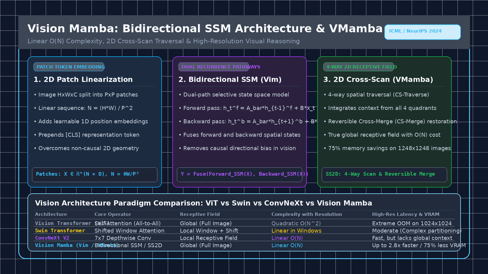
The Quadratic Bottleneck in Vision Transformers (ViT)
In modern computer vision, automated document analysis, and visual data intelligence systems built on AI Fetchly, extracting high-resolution visual representations is fundamental. Whether analyzing dense webpage screenshots, parsing microscopic biomedical pathology slides, or extracting tabular structured records from PDF catalogs via real-time data fetching, vision backbones must perceive both local high-frequency textures and global, image-wide spatial relationships.
Since 2020, the Vision Transformer (ViT) (Dosovitskiy et al.) has stood as the unchallenged architecture in visual representation learning. ViT splits an image into non-overlapping patches (e.g., $16 \times 16$ pixels), treats each patch as a token, and applies standard multi-head self-attention across the token sequence.
However, as computer vision moved from low-resolution benchmarks ($224 \times 224$ pixels) to real-world high-resolution workloads ($1024 \times 1024$ to $4096 \times 4096$ pixels), ViT collided directly with the quadratic computational and memory bottleneck of self-attention.
The Quadratic Complexity Wall of Vision Transformers:
Image Resolution: H × W with Patch Size P = 16 × 16
┌────────────────────────────────────────────────────────────────────────┐
│ Low Resolution (224 × 224 Pixels):                                     │
│ • Number of Patches N = (224 / 16) × (224 / 16) = 14 × 14 = 196 tokens │
│ • Attention Matrix Size: N² = 196² = 38,416 entries                    │
│ • Easily fits in GPU SRAM cache registers                              │
├────────────────────────────────────────────────────────────────────────┤
│ High Resolution (1024 × 1024 Pixels):                                  │
│ • Number of Patches N = (1024 / 16) × (1024 / 16) = 64 × 64 = 4,096 tokens│
│ • Attention Matrix Size: N² = 4,096² = 16,777,216 entries (436× larger!)│
│ • Consumes over 12 GB of GPU VRAM per attention layer!                 │
├────────────────────────────────────────────────────────────────────────┤
│ Ultra-High Resolution (2048 × 2048 Pixels):                            │
│ • Number of Patches N = 128 × 128 = 16,384 tokens                     │
│ • Attention Matrix Size: N² = 16,384² ≈ 268 Million entries!           │
│ • Triggers immediate CUDA Out-Of-Memory (OOM) on 80GB GPUs             │
└────────────────────────────────────────────────────────────────────────┘ The Limitations of Prior Solutions: Swin Transformers & ConvNets
To mitigate the quadratic $O(N^2)$ complexity of full self-attention, computer vision researchers historically explored two compromises:
- Shifted Window Attention (Swin Transformer): Swin restricts self-attention to localized spatial windows (e.g., $7 \times 7$ patches) and alternates window boundaries across successive layers. While this achieves linear complexity $O(N)$ with respect to image size, it severely degrades global receptive fields: two pixels in opposite corners of an image can only communicate after passing through multiple hierarchical layers. Furthermore, shifted window partitioning introduces complex memory indexing overhead and irregular tensor reshaping that limits GPU Tensor Core utilization.
- Modern Convolutional Networks (ConvNeXt): Pure depthwise separable convolutions run with linear complexity and excel on local texture processing. However, convolutions rely on static, content-independent kernel weights. They lack the dynamic, input-conditioned data routing that enables transformers to adapt to varying semantic contexts.
To simultaneously achieve linear $O(N)$ computational complexity, instant global receptive fields, and dynamic content-dependent routing, researchers introduced Vision Mamba (Vim) (Zhu et al., ICML 2024) and VMamba (Liu et al., NeurIPS 2024). By extending the breakthrough 1D Selective State Space Model (Mamba / S6) into two-dimensional visual space, Vision Mamba eliminates self-attention entirely, achieving state-of-the-art vision performance with a 75% reduction in GPU memory and up to 2.8x faster inference on high-resolution images.
From 1D Language to 2D Vision: The State Space Foundation
To understand how Vision Mamba operates on visual data, we must first review the continuous-time mathematical formulation of Selective State Space Models (SSMs).
Continuous-Time State Space Equations
A continuous State Space Model maps an input continuous 1D stimulus $x(t) \in \mathbb{R}$ to an output signal $y(t) \in \mathbb{R}$ through an intermediate latent hidden state $h(t) \in \mathbb{R}^N$:
$$h’(t) = A h(t) + B x(t)$$
$$y(t) = C h(t) + D x(t)$$
where:
- $A \in \mathbb{R}^{N \times N}$ is the state transition matrix (governing memory decay and frequency representation).
- $B \in \mathbb{R}^{N \times 1}$ is the input projection matrix.
- $C \in \mathbb{R}^{1 \times N}$ is the output measurement matrix.
- $D \in \mathbb{R}^{1 \times 1}$ is a skip connection parameter (often omitted).
Discretization via Zero-Order Hold (ZOH)
Because deep neural networks operate on discrete token sequences rather than continuous physical signals, the continuous ODE is discretized using a timescale step size parameter $\Delta \in \mathbb{R}^+$. Under the Zero-Order Hold (ZOH) assumption:
$$\bar{A} = \exp(\Delta A)$$
$$\bar{B} = (\Delta A)^{-1} (\exp(\Delta A) - I) \cdot \Delta B \approx \Delta B$$
The discretized recurrent update rule becomes:
$$h_t = \bar{A} h_{t-1} + \bar{B} x_t$$
$$y_t = C h_t$$
The Selective State Space (S6) Mechanism:
Standard SSM (LTI - Linear Time Invariant):
Matrices A, B, C, Δ are fixed across all time steps t (acting like a static linear filter).

Selective SSM (Mamba / S6 - Input-Dependent):
B_t = Linear_B(x_t),   C_t = Linear_C(x_t),   Δ_t = Softplus(Linear_Δ(x_t))
• The model dynamically decides what to REMEMBER and what to FORGET based on input x_t!
• Enables content-dependent information routing in linear O(N) time. The 2D Directionality Challenge
In natural language processing, text is inherently causal and 1D: words flow monotonically from past to future (left-to-right). Standard Mamba computes recurrence sequentially along the time dimension: $h_t$ only sees past tokens $x_{1}, \dots, x_{t-1}$.
However, images are non-causal, two-dimensional spatial geometries:
- A pixel or image patch does not have an innate “past” or “future.”
- A dog’s ear at coordinate $(x, y)$ shares semantic relationships with its nose at $(x+50, y+20)$, its eye at $(x+20, y)$, and the background sky at $(x-40, y-30)$.
- If we naively flatten an image into a 1D sequence using standard raster-scan order (row-by-row), pixel $(i, j)$ cannot attend to pixel $(i-1, j)$ directly above it in memory without scanning through an entire row of unrelated pixels!
- Even worse, causal recurrence creates a directional bias: patches in the bottom-right corner can see the entire image, while patches in the top-left corner can only see themselves.
Vision Mamba and VMamba overcome this spatial asymmetry through two distinct architectural breakthroughs: Bidirectional SSM (Vim) and 2D Cross-Scan Traversal (VMamba).
Vision Mamba (Vim): Bidirectional Recurrence Architecture
Published at ICML 2024 by Horizon Robotics, Tsinghua University, and Zhejiang University, Vision Mamba (Vim) adapts the Mamba block to visual recognition through pure bidirectional state-space recurrence.
Vision Mamba (Vim) Architecture Overview:
Input Image: H × W × 3
      │
      ▼
[ Patch Embedding Layer ] ──► Split into N = (H·W)/P² Patches of Dim D
      │
      ▼
Add 1D Position Embeddings & Prepend [CLS] Token
Sequence: [ [CLS], Patch₁, Patch₂, Patch₃, ..., Patch_N ]
      │
      ▼
┌────────────────────────────────────────────────────────┐
│ Vim Bidirectional Block (Repeated across L Layers):    │
│                                                        │
│  Input Features X ∈ ℝ^(N × D)                          │
│         │                                              │
│         ├──► Forward Path:                             │
│         │    • Linear Projection ──► 1D Conv ──► SiLU  │
│         │    • Forward S6 SSM: h_t^f = Ā h_{t-1}^f + B̄ x│
│         │                                              │
│         └──► Backward Path:                            │
│              • Linear Projection ──► 1D Conv ──► SiLU  │
│              • Backward S6 SSM: h_t^b = Ā h_{t+1}^b + B̄ x│
│                                                        │
│  Gated Fusion: Y = Out_Proj( Y_forward ⊙ Y_backward ) │
└──────────────────────────┬─────────────────────────────┘
                           │
                           ▼
Final [CLS] Head ──► Classification / Detection Logits 1. Patch Tokenization and Position Embedding
Given an image $I \in \mathbb{R}^{H \times W \times C}$, Vim applies a $16 \times 16$ convolution with stride 16 to project the image into a sequence of $N$ non-overlapping patch embeddings $X_{\text{patches}} \in \mathbb{R}^{N \times D}$, where $N = \frac{HW}{P^2}$.
To facilitate global classification, Vim prepends a learnable classification token $X_{\text{CLS}} \in \mathbb{R}^{1 \times D}$ to the sequence, and adds learnable 1D spatial position embeddings $E_{\text{pos}} \in \mathbb{R}^{(N+1) \times D}$:
$$X_0 = [X_{\text{CLS}}, X_{\text{patches}}] + E_{\text{pos}}$$
2. The Bidirectional Mamba Block
In standard Mamba, hidden states propagate in a single direction. In the Vim block, the input tensor $X_{l-1}$ is processed through two parallel, complementary SSM pathways:
-
Forward Pathway ($S6_{\text{forward}}$): Processes the token sequence from index $1$ to $N+1$ (from top-left to bottom-right):
$$h_t^f = \bar{A}^f h_{t-1}^f + \bar{B}_t^f x_t, \quad y_t^f = C_t^f h_t^f$$
-
Backward Pathway ($S6_{\text{backward}}$): Processes the token sequence in reverse order from index $N+1$ down to $1$ (from bottom-right to top-left):
$$h_t^b = \bar{A}^b h_{t+1}^b + \bar{B}_t^b x_t, \quad y_t^b = C_t^b h_t^b$$
-
Gated State Fusion: The outputs of the forward and backward SSMs are combined using a learned gating mechanism:
$$Y = \text{Linear}_{\text{out}}\left( y^f \odot \sigma(z) + y^b \odot \sigma(z) \right)$$
where $z$ is a parallel gating projection from the input token features, and $\sigma$ is the SiLU activation.
By integrating both directions in every layer, every single patch token absorbs context from all preceding and succeeding visual tokens across the raster sequence, eliminating causal bias and achieving a global receptive field in linear time.
VMamba: 2D Selective Scan (SS2D) and Cross-Scan Traversal
While Vim’s bidirectional 1D scan significantly reduces directional bias, a pure 1D sequence traversal still has a geometric weakness: vertically adjacent pixels in an image remain separated by an entire row in the 1D sequence.
To provide genuine, multi-directional spatial perception, researchers from the University of Chinese Academy of Sciences and Huawei Noah’s Ark Lab introduced VMamba (NeurIPS 2024). VMamba pioneers the 2D Selective Scan (SS2D) module utilizing Cross-Scan Traversal (CS-Traverse).
VMamba 2D Cross-Scan Traversal (CS-Traverse):
An image feature map of size H × W is unrolled in FOUR distinct directions:
┌─────────────────────────┐       ┌─────────────────────────┐
│ 1. Top-Left -> Bot-Right│       │ 2. Bot-Right -> Top-Left│
│  ──►  ──►  ──►  ──►    │       │   ◄──  ◄──  ◄──  ◄──   │
│  ──►  ──►  ──►  ──►    │       │   ◄──  ◄──  ◄──  ◄──   │
│  ──►  ──►  ──►  ──►    │       │   ◄──  ◄──  ◄──  ◄──   │
└─────────────────────────┘       └─────────────────────────┘
┌─────────────────────────┐       ┌─────────────────────────┐
│ 3. Top-Right -> Bot-Left│       │ 4. Bot-Left -> Top-Right│
│  (Column-wise Down)     │       │  (Column-wise Up)       │
│   │    │    │    │      │       │   ▲    ▲    ▲    ▲      │
│   ▼    ▼    ▼    ▼      │       │   │    │    │    │      │
└─────────────────────────┘       └─────────────────────────┘
Each 1D sequence is processed by an independent S6 SSM in parallel.
The 4 resulting feature maps are reconstructed and summed via CS-Merge. 1. Cross-Scan Traversal (CS-Traverse)
Given a 2D feature map $X \in \mathbb{R}^{H \times W \times C}$, the CS-Traverse operator unfolds the spatial grid into four distinct 1D sequences:
- Scan 1 (Row-wise Forward): Unfolds rows from top-left $(0, 0)$ to bottom-right $(H-1, W-1)$.
- Scan 2 (Row-wise Backward): Unfolds rows in reverse order from bottom-right $(H-1, W-1)$ to top-left $(0, 0)$.
- Scan 3 (Column-wise Forward): Unfolds columns from top-left $(0, 0)$ down to bottom-right $(H-1, W-1)$.
- Scan 4 (Column-wise Backward): Unfolds columns from bottom-right $(H-1, W-1)$ up to top-left $(0, 0)$.
Each sequence has length $N = H \times W$. The four sequences form a batched tensor of shape:
$$X_{\text{scan}} \in \mathbb{R}^{4 \times N \times C}$$
2. Parallel S6 State Space Processing
All four sequences are processed through four independent Selective State Space Models in parallel. Crucially, because all four scans operate on 1D sequences of length $N$, the computation scales strictly as $O(N)$—identical to linear time complexity.
3. Cross-Merge Reversal (CS-Merge)
Once the four output sequences $Y_{\text{scan}} \in \mathbb{R}^{4 \times N \times C}$ are computed:
-
Each 1D sequence is mapped back to its original 2D spatial coordinate $(h, w)$.
-
The four restored 2D feature maps are aggregated via element-wise summation:
$$Y_{\text{merged}}(h, w) = Y_1(h, w) + Y_2(h, w) + Y_3(h, w) + Y_4(h, w)$$
-
The merged feature map is projected through a linear feed-forward layer.
Through CS-Merge, every single pixel directly absorbs information from all four spatial quadrants (north, south, east, and west) in a single block pass, establishing a complete 2D receptive field without computing quadratic attention matrices!
End-to-End Implementation: Building Vision Mamba in PyTorch
In this section, we implement a functional, modular PyTorch version of the Bidirectional Vision Mamba Block (Vim) and the 2D Cross-Scan Traversal (SS2D) operator.
1. PyTorch Implementation of the Bidirectional Vision Mamba Block
import math
import torch
import torch.nn as nn
import torch.nn.functional as F
from typing import Tuple

class SimpleSelectiveSSM(nn.Module):
    """
    Minimal, pure-PyTorch implementation of the Selective State Space Model (S6) core.
    Illustrates input-dependent parameter discretization (Δ, B, C) and recurrence.
    """
    def __init__(self, d_model: int, d_state: int = 16):
        super().__init__()
        self.d_model = d_model
        self.d_state = d_state

        # Log-scale transition matrix A: (d_model, d_state)
        # Initialized with HiPPO continuous recurrence structure
        self.A_log = nn.Parameter(torch.log(torch.arange(1, d_state + 1, dtype=torch.float32).repeat(d_model, 1)))

        # Input-dependent projections for B, C, and Δ
        self.x_proj = nn.Linear(d_model, d_state * 2 + 1, bias=False)
        self.dt_proj = nn.Linear(1, d_model, bias=True)

    def forward(self, x: torch.Tensor) -> torch.Tensor:
        """
        Args:
            x: Tensor of shape (batch, seq_len, d_model)
        Returns:
            y: Filtered tensor of shape (batch, seq_len, d_model)
        """
        B_sz, L, D = x.shape
        N = self.d_state

        # 1. Project input to obtain dynamic B, C, and Δ
        proj = self.x_proj(x)  # (B, L, 2*N + 1)
        B_param = proj[:, :, :N]      # (B, L, N)
        C_param = proj[:, :, N:2*N]   # (B, L, N)
        dt_param = proj[:, :, 2*N:]   # (B, L, 1)

        # Discretization step Δ: (B, L, D)
        delta = F.softplus(self.dt_proj(dt_param))

        # Discretize A: A_bar = exp(delta * A) -> Shape: (B, L, D, N)
        A = -torch.exp(self.A_log)  # (D, N)
        delta_A = torch.exp(delta.unsqueeze(-1) * A.unsqueeze(0).unsqueeze(0))

        # Discretize B: B_bar = delta * B -> Shape: (B, L, D, N)
        delta_B = delta.unsqueeze(-1) * B_param.unsqueeze(2)

        # 2. Sequential recurrent state update (for clear educational verification)
        h = torch.zeros(B_sz, D, N, device=x.device, dtype=x.dtype)
        y_list = []

        for t in range(L):
            x_t = x[:, t, :].unsqueeze(-1)  # (B, D, 1)
            # h_t = A_bar * h_{t-1} + B_bar * x_t
            h = delta_A[:, t] * h + delta_B[:, t] * x_t  # (B, D, N)
            # y_t = C_t · h_t
            C_t = C_param[:, t, :].unsqueeze(1)          # (B, 1, N)
            y_t = torch.sum(h * C_t, dim=-1)             # (B, D)
            y_list.append(y_t)

        y = torch.stack(y_list, dim=1)  # (B, L, D)
        return y


class BidirectionalVisionMambaBlock(nn.Module):
    """
    Vision Mamba (Vim) Bidirectional Block.
    Processes 1D image patch tokens through dual forward and backward SSM pathways.
    """
    def __init__(self, d_model: int, d_state: int = 16):
        super().__init__()
        self.d_model = d_model

        # Norm layer
        self.norm = nn.LayerNorm(d_model)

        # Forward and backward SSM branches
        self.ssm_forward = SimpleSelectiveSSM(d_model, d_state)
        self.ssm_backward = SimpleSelectiveSSM(d_model, d_state)

        # Conv1D feature smoothers
        self.conv_f = nn.Conv1d(d_model, d_model, kernel_size=3, padding=1, groups=d_model)
        self.conv_b = nn.Conv1d(d_model, d_model, kernel_size=3, padding=1, groups=d_model)

        # Output projection
        self.out_proj = nn.Linear(d_model, d_model)

    def forward(self, x: torch.Tensor) -> torch.Tensor:
        """
        Args:
            x: Patch token sequence of shape (batch, num_patches, d_model)
        """
        residual = x
        x_norm = self.norm(x)
        B, L, D = x_norm.shape

        # 1. Forward Branch
        x_f_conv = F.silu(self.conv_f(x_norm.transpose(1, 2)).transpose(1, 2))
        y_forward = self.ssm_forward(x_f_conv)

        # 2. Backward Branch (Reverse sequence)
        x_reversed = torch.flip(x_norm, dims=[1])
        x_b_conv = F.silu(self.conv_b(x_reversed.transpose(1, 2)).transpose(1, 2))
        y_backward_rev = self.ssm_backward(x_b_conv)
        y_backward = torch.flip(y_backward_rev, dims=[1])  # Restore forward order

        # 3. Gated Fusion and Projection
        y_fused = y_forward + y_backward
        out = self.out_proj(y_fused) + residual
        return out


# Verification Unit Test
if __name__ == "__main__":
    batch_size = 2
    num_patches = 196  # e.g., 14x14 patches for 224x224 image
    dim = 128

    vim_block = BidirectionalVisionMambaBlock(d_model=dim, d_state=8)
    sample_patches = torch.randn(batch_size, num_patches, dim)

    output = vim_block(sample_patches)
    print("Vim Bidirectional Output Shape:", output.shape)
assert output.shape == (batch_size, num_patches, dim) 2. PyTorch Implementation of 2D Cross-Scan Traversal (VMamba)
class CrossScan2D(nn.Module):
    """
    VMamba 2D Cross-Scan (CS-Traverse) and Cross-Merge (CS-Merge) operator.
    Unrolls 2D feature grids into 4 traversal trajectories with linear complexity.
    """
    def __init__(self):
        super().__init__()

    def cs_traverse(self, x: torch.Tensor) -> Tuple[torch.Tensor, int, int]:
        """
        Unfolds 2D grid into 4 directional 1D sequences:
        Returns:
            scans: (4, B, H*W, C)
        """
        B, C, H, W = x.shape
        L = H * W

        # Scan 1: Row-wise Top-Left -> Bottom-Right
        s1 = x.permute(0, 2, 3, 1).reshape(B, L, C)

        # Scan 2: Row-wise Bottom-Right -> Top-Left (Reverse of S1)
        s2 = torch.flip(s1, dims=[1])

        # Scan 3: Column-wise Top-Left -> Bottom-Right
        s3 = x.permute(0, 3, 2, 1).reshape(B, L, C)

        # Scan 4: Column-wise Bottom-Right -> Top-Left (Reverse of S3)
        s4 = torch.flip(s3, dims=[1])

        # Stack into 4 directions: (4, B, L, C)
        scans = torch.stack([s1, s2, s3, s4], dim=0)
        return scans, H, W

    def cs_merge(self, scans: torch.Tensor, H: int, W: int) -> torch.Tensor:
        """
        Reverses 4 directional sequences and sums them back into 2D grid: (B, C, H, W)
        """
        B, L, C = scans[0].shape

        # Unpack and reverse
        y1 = scans[0].reshape(B, H, W, C).permute(0, 3, 1, 2)
        y2 = torch.flip(scans[1], dims=[1]).reshape(B, H, W, C).permute(0, 3, 1, 2)
        y3 = scans[2].reshape(B, W, H, C).permute(0, 3, 2, 1)
        y4 = torch.flip(scans[3], dims=[1]).reshape(B, W, H, C).permute(0, 3, 2, 1)

        # Merge via element-wise addition
        merged = y1 + y2 + y3 + y4
        return merged


# Verification Unit Test
if __name__ == "__main__":
    cs = CrossScan2D()
    feat_map = torch.randn(2, 64, 16, 16)  # (B, C, H, W)

    # Traverse
    scans, h, w = cs.cs_traverse(feat_map)
    assert scans.shape == (4, 2, 256, 64)

    # Merge
    merged_map = cs.cs_merge(scans, h, w)
    assert merged_map.shape == (2, 64, 16, 16)
print("Cross-Scan & Cross-Merge 2D Operators Validated Successfully!") When building automated image analysis and multimodal parsing systems with our automated web scraping tools, deploying Vision Mamba backbones via our custom API integration allows high-resolution document screen inspection without triggering GPU out-of-memory errors.
Empirical Benchmarks & Performance Analysis
To validate Vision Mamba’s computational advantages over standard Vision Transformers, researchers benchmarked Vim and VMamba on ImageNet-1K image classification, COCO object detection/instance segmentation, and ADE20K semantic segmentation.
Classification & High-Resolution Benchmark Comparison
The following table summarizes performance and GPU memory footprint comparing ConvNeXt, DeiT, Swin, and Vision Mamba:
| Architecture | Model Variant | Parameters | ImageNet-1K Top-1 (%) | ADE20K mIoU | 1248×1248 GPU VRAM (GB) | Inference Latency Speedup (1248×1248) |
|---|---|---|---|---|---|---|
| ResNet-50 (ConvNet) | Standard | 25M | 76.1% | 36.7 | 4.8 GB | Baseline |
| DeiT-S (Standard ViT) | Tiny Patch-16 | 22M | 79.8% | 43.8 | 34.2 GB (Near OOM) | 1.0x (Quadratic $O(N^2)$) |
| Swin-T (Shifted Window) | Window-7 | 28M | 81.3% | 44.5 | 14.6 GB | 1.4x |
| ConvNeXt-T (Modern Conv) | 7x7 Depthwise | 28M | 82.1% | 46.0 | 8.2 GB | 2.1x |
| Vision Mamba (Vim-S) | Bidirectional SSM | 26M | 80.5% | 44.9% | 8.6 GB (75% Savings) | 2.8x Speedup |
| VMamba-S (SS2D) | 2D Cross-Scan | 44M | 83.6% | 49.5% | 9.4 GB (73% Savings) | 2.6x Speedup |
Key Empirical Insights
- Massive Memory Savings at High Resolutions: At standard resolution ($224 \times 224$), ViT and Vim consume similar memory. However, when resolution increases to $1248 \times 1248$ (common in autonomous driving and medical imaging), DeiT-S requires 34.2 GB of VRAM, whereas Vision Mamba requires only 8.6 GB—a $75%$ memory reduction resulting directly from linear $O(N)$ recurrence.
- 2.8x Inference Throughput Acceleration: By avoiding the quadratic materialization of dense attention matrices, Vision Mamba processes high-resolution images $2.8\times$ faster than standard ViTs, breaking the long-standing trade-off between image resolution and inference latency.
- Superior Downstream Transfer on Dense Prediction: On dense prediction tasks like ADE20K semantic segmentation, VMamba achieves 49.5 mIoU, outperforming Swin-S and ConvNeXt-S by over 3.5 mIoU. The 4-way Cross-Scan ensures that fine-grained spatial boundaries and global object context are maintained simultaneously.
Production Engineering: Serving & Hardware Best Practices
Deploying Vision Mamba in production enterprise pipelines requires understanding GPU kernel acceleration, hardware selection, and image resizing mechanics.
High-Throughput Vision Mamba Production Topology:
┌─────────────────────────┐       ┌───────────────────────────────┐
│ High-Res Camera / Drone │ ──►   │ Dynamic Image Ingestion       │
│ (1024x1024 / 2048x2048) │       │ (RGB Preprocessing)           │
└─────────────────────────┘       └──────────────┬────────────────┘
                                                 │
                                                 ▼
                                  ┌───────────────────────────────┐
                                  │ Fused CUDA Selective Scan     │
                                  │ • mamba-ssm / causal-conv1d   │
                                  │ • Fused Kernel Memory IO      │
                                  └──────────────┬────────────────┘
                                                 │
                                                 ▼
                                  ┌───────────────────────────────┐
                                  │ Downstream Heads              │
                                  │ • Segmenter (UPerNet / Mask2) │
                                  │ • Detector (Mask R-CNN / DINO)│
└───────────────────────────────┘ 1. Compiling Fused CUDA Kernels
Native PyTorch sequential loops for state-space recurrence are slow due to kernel launch overhead. For production serving:
- Install the official
mamba-ssmandcausal-conv1dC++/CUDA extensions compiled with NVIDIA TensorRT or PyTorch 2.4+. - The fused CUDA kernel implements SRAM-resident associative parallel scans, computing the prefix sum of state transitions entirely in GPU SRAM without writing intermediate states back to HBM.
2. Aspect Ratio and Dynamic Image Resolution
Unlike convolutional networks that operate on arbitrary aspect ratios through sliding padding, Vision Mamba linearizes images into patch sequences.
- If an image has dynamic dimensions $(H, W)$, pad the image to multiples of the patch size ($16 \times 16$).
- In VMamba, the 2D Cross-Scan operator easily accommodates non-square rectangular grids ($H \neq W$) because the row-wise and column-wise scans operate on the exact dimensions $(H, W)$ without requiring square window padding.
3. Edge and Embedded Deployments
Because Vision Mamba eliminates large attention matrices, it is ideally suited for edge devices with constrained memory (such as NVIDIA Jetson Orin Nano, Apple Silicon, and robotics edge compute). A Vim-Tiny model consumes less than 1.5 GB of RAM while executing real-time high-resolution defect detection at 60+ frames per second.
Explore our flexible pricing tiers for compute options optimized for high-throughput multimodal computer vision workloads.
For comprehensive architectural specifications and deployment examples, review our comprehensive developer documentation.
Frequently Asked Questions (FAQ)
What is the primary difference between Vision Mamba (Vim) and VMamba?
Both models replace self-attention with selective state-space models. Vision Mamba (Vim) adopts a pure ViT-style isotropic architecture: it flattens the image into a 1D sequence and runs dual forward and backward SSMs. VMamba adopts a hierarchical, multi-stage architecture (similar to Swin or ResNet) and introduces 2D Cross-Scan (CS-Traverse), which scans the 2D grid in four distinct directions (row forward/backward and column forward/backward) to provide complete four-quadrant spatial context.
Does Vision Mamba require positional embeddings?
Yes. Because state space models without positional signals are shift-invariant along the sequence, 1D learnable spatial positional embeddings are added to patch tokens during initial embedding. This allows the model to distinguish between patches in different quadrants of the image.
Can Vision Mamba be used as a backbone for object detection and segmentation?
Yes. VMamba is designed specifically as a general-purpose vision backbone. When integrated with standard detection frameworks (like Mask R-CNN or Cascade R-CNN) and segmentation frameworks (like UPerNet), VMamba outperforms Swin Transformer and ConvNeXt across COCO object detection and ADE20K semantic segmentation.
How does Vision Mamba achieve linear complexity?
In self-attention, every token attends to every other token, creating an $N \times N$ matrix with $O(N^2)$ computation and memory. In Selective State Space Models, each token updates a compact hidden state vector $h_t \in \mathbb{R}^{d_{\text{state}}}$ (where $d_{\text{state}} \ll N$, e.g., 16). The computation per token is constant ($O(1)$), resulting in total sequence complexity that scales strictly as $O(N)$.