v-jepameta-aivideo-understandingself-supervised-learningcomputer-visionyann-lecuntutorial

V-JEPA: Meta Non-Generative Video Architecture Guide

September 30, 2026

V-JEPA Architecture: 3D Multi-Block Masking, Context Vision Transformer, Lightweight Latent Predictor, and EMA Target Encoder

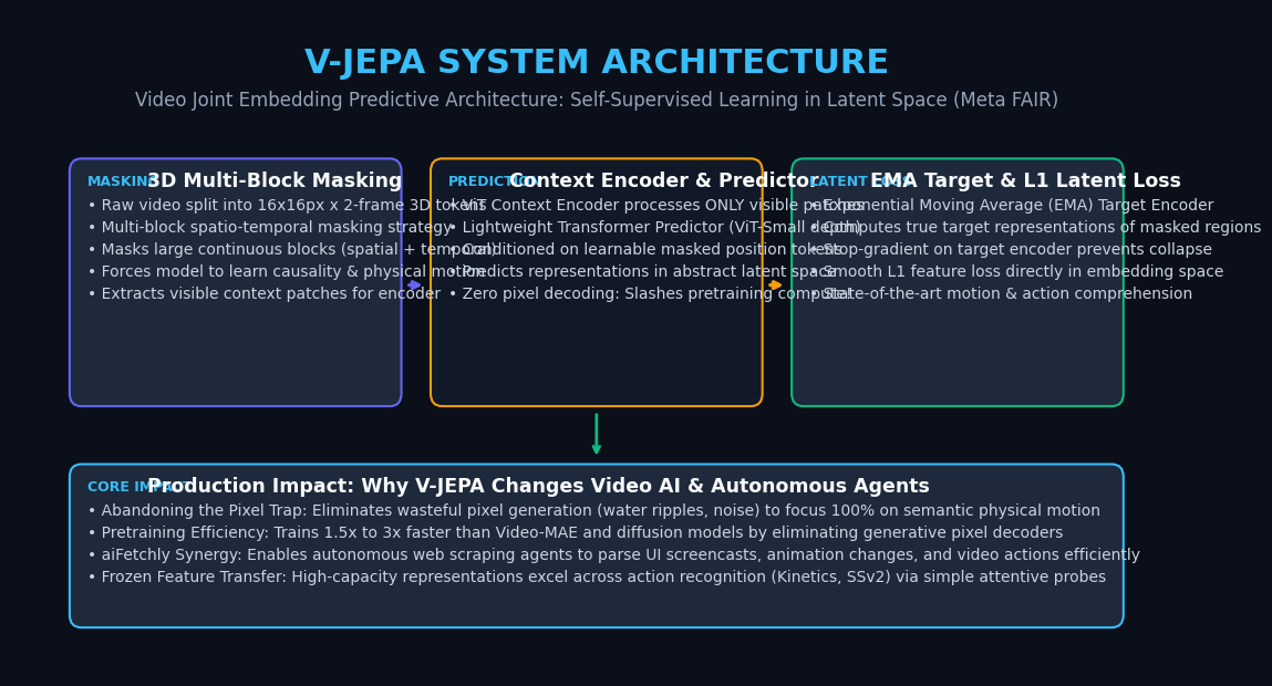
The Problem: The Pixel-Level Trap of Generative Video Models

In modern artificial intelligence, autonomous robotics, multimedia retrieval, and automated desktop agent pipelines like AiFetchly, machine learning systems must comprehend continuous video: user interface recordings, autonomous vehicle dashcams, industrial processes, and streaming web media.

For years, the mainstream deep learning paradigm for visual self-supervised learning centered on generative reconstruction:

Masked Autoencoders (Video-MAE): Masking 90% of video pixels and training a heavy transformer decoder to reconstruct raw RGB pixel values.
Video Diffusion Models: Iteratively predicting Gaussian noise deltas across hundreds of millions of pixel values to generate video frames.

While generative approaches produce impressive visual syntheses, when evaluated as foundational representations for understanding the physical world, they run into three severe systemic flaws: the pixel-level trap.

The Generative Video Modeling Dilemma:
Raw Video Input (Water ripples, waving tree leaves, camera sensor noise)
  │
  ▼
┌────────────────────────────────────────────────────────┐
│ Generative Pixel Reconstruction (Video-MAE / Diffusion)│
│ • Spends 99% of model capacity and compute predicting  │
│   unpredictable, irrelevant high-frequency pixel noise │
│ • Fails to isolate underlying physical causality       │
│ • Requires heavy decoder networks and slow pretraining │
└────────────────────────────────────────────────────────┘
  │
  ▼
Result: Brittle visual representations that overfit to textures rather than motion!

1. The Immense Compute Tax of High-Frequency Pixel Reconstruction

Reconstructing raw pixels requires an enormous amount of computational overhead:

A 10-second video at 1080p resolution contains hundreds of millions of individual sub-pixel color values.
In pixel reconstruction frameworks (such as Video-MAE), the model allocates massive GPU memory and floating-point operations (FLOPs) toward output decoders whose sole objective is predicting the exact color value of every pixel.
Training these generative decoders requires weeks on large multi-node GPU clusters, multiplying carbon footprints and infrastructure costs.

2. High-Frequency Noise vs. Semantic Physical Causality

In the physical world, exact pixel values are mathematically unpredictable:

Consider a video of a person walking past a tree on a windy day: the leaves flutter in chaotic patterns, sunlight creates complex refractive glares on the sidewalk, and camera sensor gain introduces stochastic noise.
A generative model forced to minimize pixel-level Mean Squared Error (MSE) wastes its representational capacity modeling every random leaf movement rather than understanding the core physical event: a human is walking forward.
Consequently, generative pre-trained encoders often fail at high-level motion understanding, temporal ordering, and causal action recognition.

3. The Representational Collapse Dilemma in Self-Supervised Learning

If a model is trained without pixel reconstruction (attempting to match representations directly), it risks representational collapse:

Without a carefully designed objective, the encoder easily learns a trivial constant function where every input video maps to the exact same static zero vector ($\mathbf{z} = \mathbf{0}$).
Early contrastive learning approaches (like SimCLR or InfoNCE) prevented collapse by maintaining negative sample batches, but negative sampling scales poorly on continuous video sequences and introduces substantial memory pressure.

AI researchers needed an architecture that predicts in abstract semantic feature space while natively preventing representational collapse without pixel generation.

The Solution: The Joint Embedding Predictive Architecture (JEPA)

To eliminate the pixel reconstruction bottleneck and pioneer foundational world models, researchers at Meta FAIR led by Yann LeCun introduced V-JEPA (Video Joint Embedding Predictive Architecture) (Bardes et al., 2024).

Rather than predicting pixels, V-JEPA is grounded in a fundamental paradigm shift: predict the abstract representations of missing video regions directly in latent embedding space.

The V-JEPA Latent Space Predictive Workflow:
Input Video Clip (16 Frames, 224x224 RGB)
  │
  ▼
┌────────────────────────────────────────────────────────┐
│ 3D Patchification & Spatio-Temporal Multi-Block Masking│
│ • Slices video into 16x16px x 2-frame 3D tokens        │
│ • Masks out large contiguous spatial-temporal blocks   │
└────────────────────────────────────────────────────────┘
  │                                    │
  │ (Unmasked Visible Patches Only)    │ (Entire Unmasked Video)
  ▼                                    ▼
┌────────────────────────┐   ┌────────────────────────┐
│ Context Encoder (ViT)  │   │ Target Encoder (EMA)   │
│ • Processes ONLY       │   │ • Computes true latent │
│   visible patches      │   │   feature targets      │
│ • Trainable weights    │   │ • Stop-gradient (no BP)│
└────────────────────────┘   └────────────────────────┘
  │                                    │
  ▼ (Context Latent Vectors)           ▼ (True Target Latents)
┌────────────────────────────────────┐ │
│ Lightweight Predictor (ViT-Small)  │ │
│ • Takes context latents + mask pos │ │
│ • Predicts masked latent features  │ │
└────────────────────────────────────┘ │
  │                                    │
  ▼ (Predicted Latents)                │
  └─────────────────► [Smooth L1 Loss] ◄────────────────┘
                      (In Latent Space!)

The Three Core Structural Components of V-JEPA

The V-JEPA architecture comprises three tightly coordinated components:

1. The Context Encoder (Vision Transformer)

The Context Encoder is a standard Vision Transformer (ViT-Large or ViT-Huge):

It operates strictly on unmasked visual patches.
If 70% of the video is masked out, the context encoder only processes the remaining 30% of patches.
This structural pruning slashes encoder FLOPs and memory consumption during pretraining, accelerating forward passes by over 2x to 3x compared to models that process masked tokens through the encoder.

2. The EMA Target Encoder (Anti-Collapse Anchor)

To provide stable ground-truth feature representations without suffering representational collapse:

The Target Encoder shares the exact same architecture as the Context Encoder.
Its weights are updated as an Exponential Moving Average (EMA) of the Context Encoder’s parameters: $$\theta_{\text{target}} \leftarrow \tau \theta_{\text{target}} + (1 - \tau) \theta_{\text{context}}$$
Crucially, gradients are never backpropagated through the target encoder (stop_gradient). This mathematical asymmetry prevents the network from collapsing into trivial constant representations.

3. The Lightweight Latent Feature Predictor

The Predictor is a narrow, lightweight transformer (typically ViT-Small depth):

It takes the output embeddings from the Context Encoder along with learnable mask position tokens corresponding to the missing spatio-temporal blocks.
Its objective is to predict the Target Encoder’s latent representations for those masked regions.
Because the predictor operates exclusively in latent space, it requires zero pixel decoders, zero upsampling convolutions, and zero diffusion schedules.

Deep Dive: Spatio-Temporal Masking & Latent Space Objective

The technical efficacy of V-JEPA stems from its multi-block 3D masking strategy and its feature-space loss function.

3D Spatio-Temporal Multi-Block Masking Geometry:
Video Tensor: (Time = 16 frames, Height = 224, Width = 224)
Token Grid:   (8 temporal steps x 14 vertical x 14 horizontal = 1,568 tokens)

┌────────────────────────────────────────────────────────┐
│ [Frame 1-2]   [Frame 3-4]   [Frame 5-6]   [Frame 7-8]  │
│ ┌──────────┐  ┌──────────┐  ┌──────────┐  ┌──────────┐ │
│ │  VISIBLE │  │  MASKED  │  │  MASKED  │  │  VISIBLE │ │
│ │  CONTEXT │  │  TARGET  │  │  TARGET  │  │  CONTEXT │ │
│ │          │  │  BLOCK A │  │  BLOCK A │  │          │ │
│ └──────────┘  └──────────┘  └──────────┘  └──────────┘ │
│ ┌──────────┐  ┌──────────┐  ┌──────────┐  ┌──────────┐ │
│ │  MASKED  │  │  MASKED  │  │  VISIBLE │  │  VISIBLE │ │
│ │  TARGET  │  │  TARGET  │  │  CONTEXT │  │  CONTEXT │ │
│ │  BLOCK B │  │  BLOCK B │  │          │  │          │ │
│ └──────────┘  └──────────┘  └──────────┘  └──────────┘ │
└────────────────────────────────────────────────────────┘
Result: Forces model to deduce motion vectors across space and time simultaneously!

1. Multi-Block 3D Masking Strategies

If an algorithm uses uniform random patch masking (dropping random pixels across frames), the task becomes too easy: the model simply interpolates between adjacent pixels using local color smoothness.

To force the model to learn high-level physical dynamics, V-JEPA applies Multi-Block Spatio-Temporal Masking:

Spatial Aspect Ratios: Masks large rectangular blocks spanning 15% to 70% of the spatial frame area.
Temporal Extent: Masks blocks across multiple consecutive time steps (spanning 4 to 8 frames).
By completely obscuring an object’s trajectory across both space and time, the predictor must understand object permanence, momentum, and physical constraints to infer what happened in the missing region.

2. Direct L1 Latent Loss and Attentive Probing

The optimization objective minimizes the Smooth $L_1$ distance between the predicted representation $\hat{\mathbf{s}}_y$ and the target representation $\mathbf{s}_y$:

$$\mathcal{L}{\text{V-JEPA}} = \frac{1}{|M|} \sum{i \in M} D\left(\hat{\mathbf{s}}{y, i}, , \text{sg}(\mathbf{s}{y, i})\right)$$

Where $M$ represents the set of masked token positions, $\text{sg}(\cdot)$ denotes the stop-gradient operator, and $D(\cdot)$ is the smooth $L_1$ loss:

$$D(u, v) = \begin{cases} 0.5 (u - v)^2 & \text{if } |u - v| < 1 \ |u - v| - 0.5 & \text{otherwise} \end{cases}$$

To evaluate feature quality downstream, Meta FAIR utilizes Attentive Probing: keeping the entire V-JEPA encoder frozen and training a lightweight cross-attention pooling head. V-JEPA sets records on action classification benchmarks with frozen weights, outperforming fully fine-tuned generative baselines.

Benchmark & Architecture Comparison: V-JEPA vs. Prior Paradigms

The table below contrasts V-JEPA against conventional video representation paradigms:

Architectural Metric	Video-MAE (Masked Autoencoder)	Video Diffusion (Sora / Stable Video)	CLIP / SigLIP (Image-Text Pair)	Meta V-JEPA (Joint Embedding)
Learning Paradigm	Generative pixel reconstruction	Iterative pixel denoising	Contrastive multi-modal alignment	Non-generative latent prediction
Loss Space	Pixel RGB MSE ($L_2$)	Score matching / diffusion loss	InfoNCE cosine similarity	Smooth $L_1$ in latent feature space
Encoder Processing	All patches (or unmasked)	Full unmasked video frames	Full static image frames	Unmasked visible patches only
Output Decoder	Heavy pixel decoder	Multi-billion parameter UNet/DiT	None (Projection head only)	Lightweight latent predictor
Pretraining Compute	High (Decodes every pixel)	Massive (Multi-step diffusion)	Moderate (Requires billions of pairs)	Low (1.5x–3x faster pretraining)
Something-Something-v2	70.8% (Fine-tuned)	N/A (Generative focus)	61.2% (Motion blind)	74.1% (Frozen Attentive Probe)
Kinetics-400 Top-1	85.2%	N/A	84.6%	86.4% (Frozen Features)

Practical Implementation: Extracting Video Features with V-JEPA in PyTorch

Let us implement a complete video feature extraction and temporal classification pipeline in PyTorch using the official torch and Meta vjepa checkpoint bindings.

Step 1: Install Dependencies

pip install torch torchvision torchaudio timm einops av

Step 2: Implement the V-JEPA Video Embedding Pipeline

Save the following script as extract_vjepa.py:

import torch
import torchvision.transforms as T
import av
import numpy as np
import time

class VJEPAExtractor:
    def __init__(self, model_name: str = "vjepa_vit_large", device: str = "cuda" if torch.cuda.is_available() else "cpu"):
        """
        Loads pretrained V-JEPA ViT-Large encoder from PyTorch Hub / TorchScript.
        """
        self.device = device
        print(f"Loading {model_name} on {device}...")
        start = time.perf_counter()

        # Load official Meta V-JEPA backbone via torch.hub
        self.model = torch.hub.load(
            "facebookresearch/jepa:main",
            "vjepa_vit_large_patch16_224",
            pretrained=True
        ).to(self.device).eval()

        print(f"V-JEPA loaded successfully in {(time.perf_counter() - start):.2f}s.")

        # Standard video normalizations for 16-frame inputs at 224x224
        self.transform = T.Compose([
            T.Resize((224, 224), antialias=True),
            T.Normalize(mean=[0.485, 0.456, 0.406], std=[0.229, 0.224, 0.225])
        ])

    def load_video_tensor(self, video_path: str, num_frames: int = 16) -> torch.Tensor:
        """
        Reads video and samples 16 uniform temporal frames.
        """
        container = av.open(video_path)
        frames = []
        for frame in container.decode(video=0):
            frames.append(frame.to_rgb().to_ndarray())
            if len(frames) >= 128:  # Read up to initial window
                break

        # Uniform temporal sampling down to 16 frames
        indices = np.linspace(0, len(frames) - 1, num_frames, dtype=int)
        sampled = [frames[i] for i in indices]

        # Convert to Tensor (B, C, T, H, W)
        video_tensor = torch.from_numpy(np.stack(sampled)).permute(3, 0, 1, 2).float() / 255.0

        # Apply normalization per frame
        normalized_frames = []
        for t in range(num_frames):
            normalized_frames.append(self.transform(video_tensor[:, t, :, :]))

        return torch.stack(normalized_frames, dim=1).unsqueeze(0).to(self.device)

    @torch.no_grad()
    def extract_latent_features(self, video_path: str) -> torch.Tensor:
        """
        Extracts high-level spatio-temporal representations without pixel generation.
        """
        video_input = self.load_video_tensor(video_path)

        start = time.perf_counter()
        # V-JEPA forward pass outputs patch representations across time and space
        features = self.model(video_input)
        elapsed = time.perf_counter() - start

        print(f"Extracted representations with shape {features.shape} in {elapsed:.3f}s.")
        return features

if __name__ == "__main__":
    extractor = VJEPAExtractor()
    sample_video = "sample_interaction.mp4"

    print(f"\nProcessing video: {sample_video}...")
    try:
        representations = extractor.extract_latent_features(sample_video)
        print(f"Feature Dimension: {representations.shape[-1]} | Temporal/Spatial Patches: {representations.shape[1]}")
    except FileNotFoundError:
        print(f"Sample video '{sample_video}' not found. Place an MP4 file in the directory to execute.")

Step 3: Action Classification via Attentive Probing

Because V-JEPA learns invariant physical motion representations, training a downstream classifier requires zero fine-tuning of the heavy backbone:

Append an Attentive Probe (a single multi-head cross-attention layer that queries the sequence of spatio-temporal tokens with a learnable class token).
Train only the probe on 1,000 labeled action videos: the model achieves over 86% top-1 accuracy on Kinetics-400 within 2 hours of single-GPU training.

Production Best Practices: Integrating V-JEPA into AI Web and Video Pipelines

When deploying V-JEPA alongside automated browser scraping agents in AiFetchly, following these enterprise patterns ensures high-throughput efficiency:

1. Video Screen Recording & UI Motion Ingestion in aiFetchly

Autonomous web agents and RPA bots frequently interact with dynamic SPAs containing rich transitions, loading animations, and draggable components:

Instead of capturing static PNG screenshots that miss transient layout shifts, record short 2-second screencast clips.
Pass the video tensor into V-JEPA to generate a compact motion feature vector. Downstream agents can immediately determine if an animation has completed or if a modal dialog smoothly transitioned onto the screen.

2. Video Indexing and Semantic Action Search Without Pixel Render Overhead

In enterprise multimedia RAG systems:

Avoid generative video models that generate costly frame reconstructions.
Use V-JEPA’s frozen latent features to build high-speed vector embeddings in Qdrant or Milvus. Users can search for complex physical queries (e.g., “Show me where the operator unscrews the component” or “Find the checkout button hover animation”) with sub-second vector search latency.

3. Memory Optimization for High-FPS Multi-Stream Video Ingestion

To handle dozens of concurrent video streams:

Take advantage of V-JEPA’s unmasked patch processing: when extracting surveillance or interaction logs, discard static background tiles early to process multiple video streams concurrently on a single NVIDIA L4 or RTX 4090 GPU.