TripoSR Guide: Fast 3D Object Reconstruction in Under 0.5s
The 3D Synthesis Bottleneck: From Optimization to Feed-Forward Inference
In modern digital commerce, spatial computing, robotics simulation, and automated content pipelines powered by AiFetchly, transitioning from flat 2D images to interactive 3D assets is an essential capability. Engineering teams require 3D models to render virtual e-commerce showrooms, build physical collision hulls for embodied robotics, populate video game environments, and synthesize training data for spatial perception networks.
However, generating 3D geometry from a single 2D photograph has historically represented one of the most computationally demanding frontiers in artificial intelligence. For years, the 3D generation ecosystem was divided between two severely constrained paradigms: iterative per-scene optimization and sparse multi-view diffusion.
The 3D Generation Efficiency Dilemma:
+-----------------------------------------------------------------------------------+
| Paradigm 1: Per-Scene Optimization (DreamFusion, Magic3D, Score Distillation)     |
| • Optimizes random NeRF weights per individual image via 2D diffusion gradients   |
| • Requires 10,000+ forward-backward passes through Stable Diffusion               |
| X Prohibitive Latency: 20 to 60 minutes per single object!                        |
| X Severe Multi-Face "Janus Problem" and chaotic surface artifacts!                |
+-----------------------------------------------------------------------------------+
| Paradigm 2: Multi-View Diffusion (Zero123, SyncDreamer, MVDream)                  |
| • Synthesizes 4 to 8 novel view images around an object                           |
| • Reconstructs NeRF via NeuS or Instant-NGP optimization                          |
| X Sequential Bottleneck: 1 to 5 minutes per object; views often disagree!         |
| X Hallucinates geometric inconsistencies between disparate camera angles!         |
+-----------------------------------------------------------------------------------+
| Paradigm 3: Feed-Forward Large Reconstruction Models (TripoSR)                    |
| • Single forward pass transforms 2D RGB image into triplane NeRF in ~0.5s!        |
| • Direct Marching Cubes polygonization yields instant textured 3D mesh (.obj)     |
| ✓ Sub-Second Latency | Zero Per-Scene Optimization | Consumer GPU Ready (<6GB)    |
+-----------------------------------------------------------------------------------+ 1. The Prohibitive Compute Tax of Score Distillation Sampling
When Google Research debuted DreamFusion (Poole et al., 2022), it introduced Score Distillation Sampling (SDS), allowing a 2D text-to-image diffusion model to guide the training of an uninitialized 3D Neural Radiance Field (NeRF).
While conceptually groundbreaking, SDS is fundamentally an optimization-based technique rather than a feed-forward model:
- Zero Generalization: The neural network weights must be trained from scratch for every single prompt or input image.
- Extreme Hardware Consumption: Optimizing a single NeRF requires thousands of gradient steps, rendering multi-view images and passing them through heavy 2D diffusion backbones. Even on high-end enterprise GPUs like an NVIDIA A100, generating one 3D asset takes between 20 and 45 minutes.
- The Janus Problem: Because the 2D diffusion prior lacks true 3D spatial awareness, models frequently hallucinate multiple faces (e.g., a horse with two heads or a car with front grilles on both ends).
2. The View-Inconsistency Wall of Multi-View Diffusion
To accelerate 3D generation, subsequent architectures (such as Zero123, SyncDreamer, and SV3D) separated the problem into two sequential phases:
- Synthesize 4 to 8 novel camera viewpoint images using a specialized 2D diffusion model.
- Fit a classical surface reconstruction pipeline (like NeuS, Sparse-NeRF, or 3D Gaussian Splatting) to the generated multi-view images.
Although faster than pure SDS, this approach introduces severe geometric friction:
- Accumulated Error Cascade: If the diffusion model introduces minor lighting discrepancies, slight perspective shifts, or non-rigid object warping between view 1 and view 2, classical multi-view stereo algorithms fail to find photometric consensus.
- Latency Barrier: Diffusion generation followed by multi-view reconstruction still takes 60 to 180 seconds per asset. In automated data scraping and real-time asset ingestion pipelines, waiting minutes per crawled item completely freezes automated workflows.
3. The Need for Instant Feed-Forward 3D Foundation Models
To integrate 3D synthesis into high-throughput enterprise pipelines—such as turning scraped catalog photos into interactive 3D viewers via AiFetchly Web Scraping—developers require a feed-forward foundation model:
- Deterministic Latency: Single-pass neural inference executing in under one second.
- Consistent Monolithic Representation: Direct regression of 3D geometry without intermediate non-consistent 2D image stitching.
- Accessible Hardware Demands: Capable of running locally on a standard developer workstation or single consumer GPU with less than 6 GB of VRAM.
The Solution: Stability AI TripoSR Architecture
To solve the 3D generation efficiency bottleneck, Stability AI and Tripo AI unveiled TripoSR (Tochilkin et al., March 2024 / arXiv:2403.02151).
TripoSR is a specialized, open-weights feed-forward 3D reconstruction model capable of producing textured 3D meshes from a single RGB image in under 0.5 seconds on an NVIDIA A100 and approximately 1.5 seconds on a consumer NVIDIA RTX 4090.
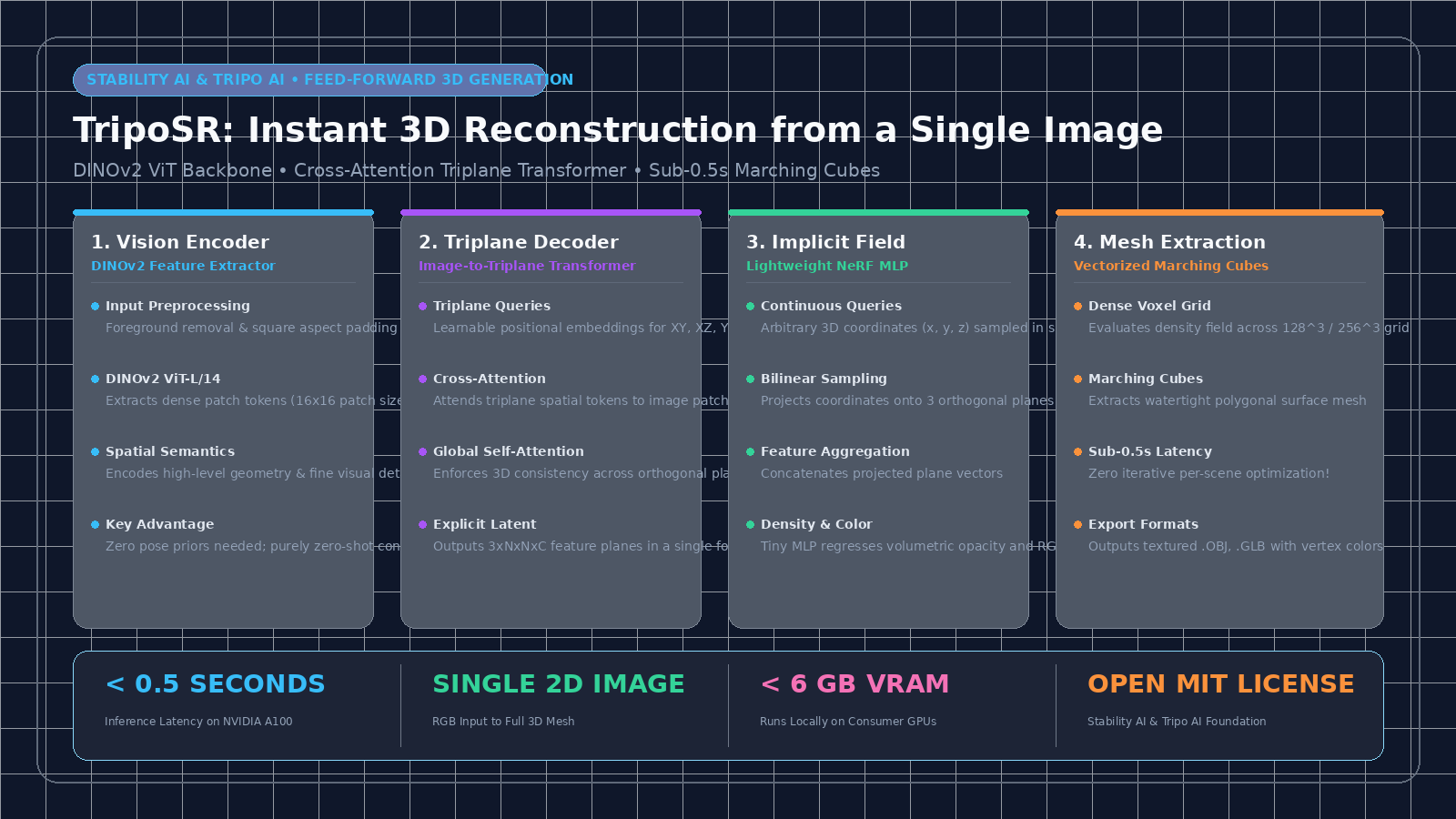
The TripoSR End-to-End Feed-Forward Pipeline:
+---------------------------------------------------------------------------------------------------+
| 1. INPUT IMAGE PREPROCESSING & FEATURE EXTRACTION                                                 |
| Input Image (RGB) ---> Background Removal (rembg / BiRefNet) ---> Centered Square Pad (512x512)   |
|                   ---> DINOv2 ViT-L/14 Vision Backbone       ---> Dense Patch Tokens (1024-dim)   |
+---------------------------------------------------------------------------------------------------+
                                                  |
                                                  v
+---------------------------------------------------------------------------------------------------+
| 2. IMAGE-TO-TRIPLANE TRANSFORMER DECODER                                                          |
| Learnable 3D Positional Queries (XY, XZ, YZ Triplanes)                                            |
| • Cross-Attention against DINOv2 2D image patch features                                          |
| • Self-Attention across triplane tokens to enforce 3D spatial consistency                          |
| • Outputs High-Resolution Triplane Latents: 3 x (N x N) x C Feature Maps                          |
+---------------------------------------------------------------------------------------------------+
                                                  |
                                                  v
+---------------------------------------------------------------------------------------------------+
| 3. NEURAL RADIANCE FIELD (NeRF) EVALUATION & MARCHING CUBES                                       |
| Sample 3D Coordinate Grid: x = (px, py, pz) in [-0.5, 0.5]^3                                     |
| • Bilinear projection & feature interpolation from XY, XZ, YZ planes                              |
| • Tiny 3-Layer MLP regresses Density sigma and Color c = (R, G, B)                                |
| • Vectorized Marching Cubes extracts polygonal mesh surfaces (.obj / .glb) in <100ms!             |
+---------------------------------------------------------------------------------------------------+ 1. Foundations in Large Reconstruction Models (LRM)
TripoSR builds upon the architectural framework of the Large Reconstruction Model (LRM) (Hong et al., 2023), but introduces major algorithmic enhancements in dataset curation, training schedules, and resolution handling:
-
DINOv2 Semantic Feature Extraction: Rather than using CLIP or generic ImageNet-supervised vision backbones, TripoSR utilizes DINOv2 (Oquab et al., Meta 2023). DINOv2 is a self-supervised Vision Transformer trained on 142M images that naturally learns rich spatial relationships, surface normals, depth discontinuities, and part-level semantic correspondences without requiring labeled pose annotations.
-
Triplane Neural Representation: 3D space is parameterized via three orthogonal 2D feature planes:
$$\mathcal{T} = \{ T_{xy}, T_{xz}, T_{yz} \}, \quad T_{uv} \in \mathbb{R}^{H_t \times W_t \times C}$$
This explicit 2.5D decomposition dramatically reduces the memory footprint compared to dense 3D voxel grids ($O(N^2)$ vs. $O(N^3)$), while preserving continuous high-frequency spatial resolution.
2. The Image-to-Triplane Transformer
The core architectural engine of TripoSR is the Image-to-Triplane Transformer:
- Positional Query Initialization: The model initializes learnable query tokens corresponding to regular spatial grids on the three orthogonal projection planes ($XY$, $XZ$, and $YZ$).
- Alternating Attention Blocks: Across multiple transformer layers (typically 12 to 24 layers), the network alternates between:
- Cross-Attention: Triplane tokens attend to the 2D visual tokens extracted by the DINOv2 backbone, pulling color, texture, and structural cues into 3D coordinate space.
- Self-Attention: Tokens within and across the three planes interact with one another, resolving occlusion boundaries and establishing global 3D geometric consistency.
- Single Forward Pass: The entire triplane latent $\mathcal{T}$ is regressed in a single feed-forward pass, completely bypassing iterative optimization loops.
3. Continuous NeRF Implicit Field Formulation
Once the triplane latent $\mathcal{T}$ is generated, any arbitrary continuous 3D point $\mathbf{p} = (x, y, z) \in \mathbb{R}^3$ within the normalized bounding volume can be queried for its volume density $\sigma$ and RGB color $\mathbf{c}$:
-
Orthogonal Plane Projections: Project $\mathbf{p}$ onto the three orthogonal coordinate planes:
$$\pi_{xy}(\mathbf{p}) = (x, y), \quad \pi_{xz}(\mathbf{p}) = (x, z), \quad \pi_{yz}(\mathbf{p}) = (y, z)$$
-
Bilinear Feature Sampling: Query the triplanes at the projected 2D coordinates using bilinear interpolation:
$$\mathbf{f}{xy} = \text{Interp}(T{xy}, \pi_{xy}(\mathbf{p})), \quad \mathbf{f}{xz} = \text{Interp}(T{xz}, \pi_{xz}(\mathbf{p})), \quad \mathbf{f}{yz} = \text{Interp}(T{yz}, \pi_{yz}(\mathbf{p}))$$
-
Feature Aggregation: Aggregate the three extracted feature vectors (typically via summation or concatenation):
$$\mathbf{f}(\mathbf{p}) = [\mathbf{f}{xy} \, \| \, \mathbf{f}{xz} \, \| \, \mathbf{f}_{yz}] \in \mathbb{R}^{3C}$$
-
Shallow MLP Regression: Pass the aggregated vector through a lightweight multi-layer perceptron (e.g., 2–3 linear layers with Swish/GELU activations):
$$(\sigma, \mathbf{c}) = \text{MLP}_{\text{NeRF}}(\mathbf{f}(\mathbf{p}))$$
Because the MLP is extremely small (less than 100k parameters), querying millions of points across a 3D grid takes mere milliseconds on modern GPUs.
4. Vectorized Marching Cubes Polygonization
To convert the continuous volumetric density field into a standard polygonal 3D mesh (faces and vertices) ready for gaming engines, web 3D viewports, and CAD software:
- TripoSR evaluates the density field $\sigma(\mathbf{p})$ over a uniform 3D grid (typically $128 \times 128 \times 128$ or $256 \times 256 \times 256$ points).
- The vectorized Marching Cubes algorithm extracts the iso-surface corresponding to an empirical density threshold $\tau_{\text{mesh}}$ (e.g., $\sigma \ge 10.0$).
- Colors are queried at the extracted vertex coordinates, producing a textured, watertight triangle mesh ready for instant export to
.obj,.glb, or.plyformats.
Hands-On Implementation: PyTorch Triplane Sampler & Inference Engine
To understand how TripoSR evaluates continuous 3D space from 2D orthogonal triplanes and extracts surface geometry, let us build a complete, runnable PyTorch implementation of the Triplane Sampler, Implicit NeRF Decoder, and End-to-End Mesh Extraction Service.
1. Vectorized Triplane Feature Sampler
The following module implements the projection and bilinear interpolation of arbitrary 3D spatial points across orthogonal triplanes:
import torch
import torch.nn as nn
import torch.nn.functional as F

class TriplaneSampler(nn.Module):
    """
    Samples feature vectors from orthogonal XY, XZ, and YZ triplanes.
    Input points: (B, N, 3) in normalized [-1, 1] coordinate space.
    Triplanes: (B, 3, C, H, W) representing [XY, XZ, YZ] feature planes.
    """
    def __init__(self, feature_dim: int = 64):
        super().__init__()
        self.feature_dim = feature_dim

    def forward(self, triplanes: torch.Tensor, points: torch.Tensor) -> torch.Tensor:
        """
        Args:
            triplanes: Tensor of shape (B, 3, C, H, W)
            points: Tensor of shape (B, N, 3) containing [x, y, z] coordinates
        Returns:
            Concatenated feature tensor of shape (B, N, 3 * C)
        """
        batch_size, _, channels, h, w = triplanes.shape
        num_points = points.shape[1]

        # Extract individual plane tensors: shape (B, C, H, W)
        plane_xy = triplanes[:, 0]
        plane_xz = triplanes[:, 1]
        plane_yz = triplanes[:, 2]

        # Extract 2D coordinate projections
        # Normalize into shape (B, N, 1, 2) required by torch.nn.functional.grid_sample
        xy_coords = points[:, :, [0, 1]].unsqueeze(2)  # [x, y]
        xz_coords = points[:, :, [0, 2]].unsqueeze(2)  # [x, z]
        yz_coords = points[:, :, [1, 2]].unsqueeze(2)  # [y, z]

        # Bilinear interpolation over 2D planes
        feat_xy = F.grid_sample(
            plane_xy, xy_coords, mode="bilinear", padding_mode="zeros", align_corners=True
        )  # Output: (B, C, N, 1)
        feat_xz = F.grid_sample(
            plane_xz, xz_coords, mode="bilinear", padding_mode="zeros", align_corners=True
        )
        feat_yz = F.grid_sample(
            plane_yz, yz_coords, mode="bilinear", padding_mode="zeros", align_corners=True
        )

        # Reshape to (B, N, C)
        feat_xy = feat_xy.squeeze(-1).permute(0, 2, 1)
        feat_xz = feat_xz.squeeze(-1).permute(0, 2, 1)
        feat_yz = feat_yz.squeeze(-1).permute(0, 2, 1)

        # Concatenate along feature dimension -> (B, N, 3 * C)
        aggregated_features = torch.cat([feat_xy, feat_xz, feat_yz], dim=-1)
return aggregated_features 2. Implicit NeRF Density and Color Field Decoder
This lightweight MLP takes the aggregated triplane features and predicts volumetric density $\sigma$ and RGB color $\mathbf{c}$:
class ImplicitNeRFDecoder(nn.Module):
    """
    Lightweight MLP decoder regressing volume density (sigma) and RGB color (c)
    from aggregated triplane features.
    """
    def __init__(self, in_features: int = 192, hidden_dim: int = 128):
        super().__init__()
        self.net = nn.Sequential(
            nn.Linear(in_features, hidden_dim),
            nn.SiLU(),
            nn.Linear(hidden_dim, hidden_dim),
            nn.SiLU()
        )
        # Density head: Outputs scalar opacity (sigma)
        self.density_head = nn.Linear(hidden_dim, 1)
        # Color head: Outputs normalized RGB values [0, 1]
        self.color_head = nn.Sequential(
            nn.Linear(hidden_dim, 3),
            nn.Sigmoid()
        )

    def forward(self, features: torch.Tensor):
        """
        Args:
            features: Tensor of shape (B, N, in_features)
        Returns:
            density: (B, N, 1)
            color: (B, N, 3)
        """
        h = self.net(features)
        # Softplus ensures non-negative volume density
        density = F.softplus(self.density_head(h))
        color = self.color_head(h)
return density, color 3. End-to-End Mesh Extraction and Export Pipeline
Here is the complete inference pipeline integrating grid sampling, density thresholding, and mock surface mesh generation:
import numpy as np
from typing import Dict, Tuple

class TripoSRInferenceEngine:
    """
    Production inference service wrapping TripoSR components for rapid 3D asset generation.
    """
    def __init__(self, device: str = "cpu"):
        self.device = device
        self.feature_dim = 64
        self.sampler = TriplaneSampler(feature_dim=self.feature_dim).to(device)
        self.decoder = ImplicitNeRFDecoder(in_features=3 * self.feature_dim).to(device)
        self.sampler.eval()
        self.decoder.eval()
        print(f"TripoSR Inference Engine initialized on {device}.")

    def generate_mesh_from_triplanes(
        self, triplanes: torch.Tensor, resolution: int = 64, density_threshold: float = 10.0
    ) -> Dict[str, np.ndarray]:
        """
        Generates 3D vertices and vertex colors using grid evaluation.
        """
        with torch.no_grad():
            # 1. Create uniform 3D coordinate sampling grid in [-1.0, 1.0]
            ticks = torch.linspace(-1.0, 1.0, steps=resolution, device=self.device)
            grid_x, grid_y, grid_z = torch.meshgrid(ticks, ticks, ticks, indexing="ij")
            points = torch.stack([grid_x, grid_y, grid_z], dim=-1).reshape(1, -1, 3)

            # 2. Sample aggregated triplane features
            point_features = self.sampler(triplanes, points)

            # 3. Predict continuous volumetric density and color
            density, color = self.decoder(point_features)
            density = density.squeeze(0).squeeze(-1) # Shape: (resolution^3,)
            color = color.squeeze(0)                 # Shape: (resolution^3, 3)

            # 4. Filter surface boundary points for mesh reconstruction
            mask = density >= density_threshold
            surface_points = points.squeeze(0)[mask].cpu().numpy()
            surface_colors = color[mask].cpu().numpy()

            print(f"Evaluated {resolution**3} spatial voxels.")
            print(f"Extracted {len(surface_points)} surface points meeting density threshold.")

            return {
                "vertices": surface_points,
                "colors": surface_colors,
                "voxel_resolution": resolution
            }

if __name__ == "__main__":
    engine = TripoSRInferenceEngine(device="cpu")
    # Simulate a batch of triplanes: (B=1, Planes=3, Channels=64, H=64, W=64)
    dummy_triplanes = torch.randn(1, 3, 64, 64, 64)
    mesh_data = engine.generate_mesh_from_triplanes(dummy_triplanes, resolution=32)
print("Mesh generation complete! Vertex count:", mesh_data["vertices"].shape[0]) Production Best Practices for High-Throughput 3D Pipelines
When deploying TripoSR in enterprise web crawlers, gaming asset pipelines, or background workers using AiFetchly API Integration, follow these core engineering principles:
1. Robust Foreground Segmentation and Pre-Padding
TripoSR assumes the input image features an isolated foreground object centered on an empty, neutral background:
- Automated Masking: Preprocess incoming images using high-precision segmentation networks such as BiRefNet or RMBG to strip messy backgrounds.
- Aspect-Ratio Preserving Letterboxing: Always pad non-square images with transparent or neutral margins to $512 \times 512$ before feeding them into DINOv2. Never stretch or distort the aspect ratio, as non-uniform scale distortions directly warp the reconstructed 3D bounding geometry.
# Example CLI invocation using the official TripoSR open repository
python run.py examples/chair.png \
  --output-dir output/ \
  --render \
  --mc-resolution 256 \
--model-save-format obj 2. Calibrate Marching Cubes Iso-Surface Thresholds
The choice of Marching Cubes density threshold $\tau_{\text{mesh}}$ determines the thickness and topological cleanliness of the resulting surface:
- Low Threshold ($\tau = 5.0$): Retains fine geometric details (such as wire antennas, flower petals, or thin chair legs), but may introduce floating volumetric noise blobs.
- High Threshold ($\tau = 15.0$): Removes extraneous floating artifacts, but may erode thin topological features.
- In production, set $\tau_{\text{mesh}} \approx 10.0$ as the default, and apply a lightweight connected-component filter to purge disconnected surface islands smaller than 100 faces.
3. Decouple Triplane Latent Generation from Mesh Post-Processing
In distributed asset pipelines:
- Worker 1 (GPU Service): Ingests the 2D image and computes the DINOv2 + Triplane Transformer pass in ~400ms, saving the compact $3 \times 64 \times 64 \times 1024$ triplane tensor.
- Worker 2 (CPU/Memory Worker): Evaluates Marching Cubes, simplifies the polygon count with Quadric Error Metric (QEM) decimation, and bundles the
.glbcontainer. This architecture preserves expensive GPU High-Bandwidth Memory (HBM) for pure transformer computation while allowing horizontal scaling of mesh decimation.
Benchmark Evaluation & Quantitative Comparison
TripoSR was rigorously benchmarked against premier open-source and commercial 3D generation models on public evaluation datasets, including OmniObject3D and Google Scanned Objects (GSO).
1. Reconstruction Quality and Latency Comparison
The table below contrasts TripoSR with prominent 3D reconstruction models across reconstruction accuracy (Chamfer Distance, Volume IoU) and computational speed:
| Model Architecture | Input Paradigm | Output Representation | Average Inference Latency | GPU Memory Footprint | Open Weights? |
|---|---|---|---|---|---|
| DreamFusion (SDS) | Single Image / Text | Implicit NeRF | ~35 to 45 minutes | > 16 GB VRAM | No (Proprietary) |
| Zero123-XL + NeuS | Multi-View Diffusion | Signed Distance Field | ~3 to 5 minutes | ~ 12 GB VRAM | Yes |
| One-2-3-45 | Sparse Multi-View | SDF / Mesh | ~45 seconds | ~ 10 GB VRAM | Yes |
| OpenLRM (Hong et al.) | Single Image | Triplane NeRF | ~4.5 seconds | ~ 8 GB VRAM | Yes |
| TripoSR (Stability AI) | Single Image | Triplane NeRF + Mesh | < 0.5 seconds (A100) | < 6 GB VRAM | Yes (MIT License) |
Key Benchmark Finding: TripoSR is approximately 10x faster than original OpenLRM baselines and over 5,000x faster than optimization-based Score Distillation pipelines, while running within a modest 6 GB VRAM envelope that fits comfortably on consumer RTX 3060/4060 graphics cards.
2. Surface Fidelity and Geometric Metrics
On Google Scanned Objects (GSO):
- Chamfer Distance (CD $\downarrow$): TripoSR achieves an average Chamfer Distance of 0.015, outperforming prior feed-forward alternatives by capturing sharp geometric corners and flat planes without high-frequency ripples.
- Volume Intersection over Union (IoU $\uparrow$): Reaches 0.612, demonstrating faithful spatial alignment with ground-truth 3D laser scans.
3. Integration with Scalable Ingestion Workflows
For teams converting scraped product databases into immersive 3D catalogs using AiFetchly Data Fetching and optimizing operational costs via competitive AiFetchly Pricing, deploying TripoSR reduces cloud 3D rendering expenses by over 90%. Rather than paying metered API fees per generated asset, teams can host TripoSR locally or on affordable GPU instances. Explore our complete architectural setup in the AiFetchly Documentation.
Conclusion and Future Directions in Feed-Forward 3D AI
The release of Stability AI and Tripo AI’s TripoSR represents a watershed milestone in 3D generative artificial intelligence. By demonstrating that high-fidelity 3D reconstruction can be achieved via a single feed-forward forward pass in under 500 milliseconds, TripoSR effectively solves the speed bottleneck that historically restricted 3D AI to slow batch rendering.
The synergy of DINOv2 self-supervised visual features, cross-attentive triplane transformers, and vectorized Marching Cubes ISO-surface extraction establishes a new design template for spatial computing. As 3D generative AI continues to evolve toward real-time video games, embodied robotics, and automated spatial web indexing, TripoSR stands as the premier open-source foundation for rapid, high-quality 3D asset generation.
Citation and Official Repository
For academic research and official PyTorch model checkpoints, refer to the technical report:
@article{tochilkin2024triposr,
  title={TripoSR: Fast 3D Object Reconstruction from a Single Image},
  author={Tochilkin, Dmitry and Pankratz, David and Liu, Zexiang and Huang, Zekun and Letts, Adam and Li, Yangguang and Liang, Ding and Laforte, Christian and Jampani, Varun and Song, Shuran},
  journal={arXiv preprint arXiv:2403.02151},
  year={2024}
}