Token Merging (ToMe) Guide: 2x Faster ViT & Diffusion Models
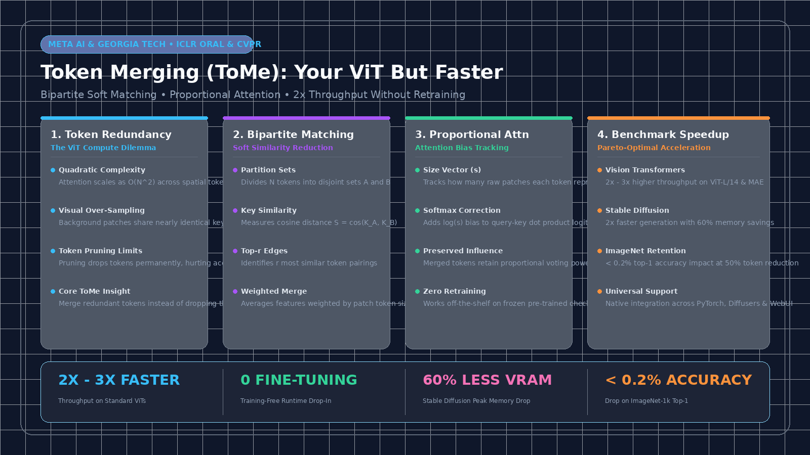
The Quadratic Cost of Visual Redundancy in Modern Transformers
In modern desktop AI assistants, high-throughput media analysis, visual scraping pipelines, and automated intelligence platforms powered by AiFetchly, transformer architectures have become the universal foundation across computer vision and multimodal synthesis. Whether classifying crawled e-commerce products using Vision Transformers (ViT), indexing multi-modal web assets with CLIP, or generating high-resolution synthetic imagery via Stable Diffusion, transformer backbones deliver state-of-the-art representational power.
However, the computational mechanics of self-attention impose a severe throughput and memory tax when applied to images:
The Visual Token Scaling Wall:
+-----------------------------------------------------------------------------------+
| 1. Quadratic Self-Attention Complexity: O(N^2)                                    |
| • Standard ViT divides an image into N spatial patch tokens (e.g., 196 to 1024)   |
| • Full all-to-all attention scales quadratically with sequence length             |
| X Computing pairwise attention across dense grids exhausts GPU memory bandwidth!  |
+-----------------------------------------------------------------------------------+
| 2. Pervasive Visual Redundancy                                                    |
| • Unlike text words, neighboring image patches in background regions (sky, walls, |
|   empty backgrounds, textures) share nearly identical semantic representations    |
| X Standard models expend >60% of total FLOPs recalculating identical features!    |
+-----------------------------------------------------------------------------------+
| 3. The Pitfalls of Token Pruning                                                  |
| • Prior compression methods drop "unimportant" tokens permanently                 |
| • Hard token dropping discards subtle peripheral cues and alters sequence lengths |
| X Triggers catastrophic accuracy degradation without extensive model re-training! |
+-----------------------------------------------------------------------------------+ 1. The Quadratic Scaling Dilemma in Vision
In natural language processing, each token represents a distinct subword unit with unique morphological and semantic properties. In computer vision, however, images are continuous 2D signals:
- When a Vision Transformer slices a $224 \times 224$ image into $16 \times 16$ patches, it creates $196$ spatial tokens.
- At higher resolutions (such as $512 \times 512$ in Stable Diffusion or $1024 \times 1024$ in document parsing), the token count explodes to 1,024 to 4,096 tokens per image.
- Because the self-attention operation computes pairwise dot products across all tokens:
$$\text{Attention}(Q, K, V) = \text{Softmax}\left(\frac{Q K^\top}{\sqrt{d_k}}\right) V$$
Computing attention requires $O(N^2)$ FLOPs and materializes large intermediate attention matrices in High-Bandwidth Memory (HBM). When batching thousands of downloaded product photos via AiFetchly Web Scraping, this quadratic wall caps server throughput and inflates cloud inference costs.
2. High Spatial Redundancy in Visual Information
A fundamental property of natural images is spatial continuity:
- In an image of a cat resting on a hardwood floor, dozens of image patches correspond to uniform wood grain, blank background wall, or smooth fur.
- After early transformer layers encode low-level textures, the feature vectors of these adjacent patches become virtually identical in latent space ($\cos(x_i, x_j) > 0.95$).
- In standard architectures, these redundant tokens continue to propagate through all 24 or 32 subsequent transformer layers, consuming valuable matrix multiplication compute and register bandwidth without adding new information.
3. Why Token Pruning Falls Short
To reduce token counts, early research focused on Token Pruning (e.g., DynamicViT, EViT):
- Permanent Information Loss: Pruning scores tokens by attention weights or class relevance and completely deletes the lowest-scoring tokens. If a pruned token contains a small but critical detail (such as a tiny button, logo, or edge boundary), that information is permanently vanished from all downstream layers.
- Retraining Requirement: Because sudden deletion of tokens alters the hidden state distribution, pruned models suffer severe performance collapse unless subjected to multi-epoch fine-tuning with complex masking schedules.
- Architectural Brittleness in Generative Models: In generative diffusion models (like Stable Diffusion), dropping spatial tokens creates visible holes, distorted object boundaries, and blurred textures in the synthesized output.
The Solution: Token Merging (ToMe) Architecture
To eliminate visual redundancy without the drawbacks of token pruning, Meta AI and Georgia Tech (Bolya et al., ICLR 2023 oral) introduced Token Merging (ToMe).
Rather than deleting tokens, ToMe merges redundant tokens together using an efficient bipartite matching algorithm. By combining similar tokens and tracking their accumulated information mass, ToMe accelerates existing pre-trained Vision Transformers and Diffusion models by 2x to 3x with zero fine-tuning or training required.
The Token Merging (ToMe) Algorithmic Pipeline:
+---------------------------------------------------------------------------------------------------+
| 1. PARTITION TOKENS INTO BIPARTITE SETS                                                           |
| Input Sequence: X in R^(N x D) ---> Deterministic Alternating Split: Set A (N/2) and Set B (N/2)  |
+---------------------------------------------------------------------------------------------------+
                                                  |
                                                  v
+---------------------------------------------------------------------------------------------------+
| 2. BIPARTITE SOFT MATCHING (BSM)                                                                  |
| • Extract Keys: K_A in Set A, K_B in Set B                                                        |
| • Compute Cosine Similarity Matrix: S = (K_A / ||K_A||) @ (K_B / ||K_B||)^T                       |
| • For each token in A, find most similar partner in B: argmax_j S_{i, j}                          |
| • Select top-r most similar edges across the entire bipartite graph                               |
+---------------------------------------------------------------------------------------------------+
                                                  |
                                                  v
+---------------------------------------------------------------------------------------------------+
| 3. WEIGHTED FEATURE REDUCTION & SIZE ACCUMULATION                                                 |
| For each selected pair (a in A -> b in B):                                                        |
| • Merged Feature: x_b' = (s_a * x_a + s_b * x_b) / (s_a + s_b)                                    |
| • Accumulated Size: s_b' = s_a + s_b (Tracks original patch count)                                |
| Sequence Length: Reduced from N tokens to (N - r) tokens in a single transformer block!           |
+---------------------------------------------------------------------------------------------------+
                                                  |
                                                  v
+---------------------------------------------------------------------------------------------------+
| 4. PROPORTIONAL ATTENTION (DOWNSTREAM ATTENTION CORRECTION)                                       |
| In subsequent attention layers: Add log(s) bias to query-key logits:                             |
| Softmax((Q @ K^T) / sqrt(d) + log(s)) @ V                                                         |
| Merged tokens retain their correct democratic influence across the entire transformer!            |
+---------------------------------------------------------------------------------------------------+ 1. Bipartite Soft Matching (BSM)
The central algorithmic breakthrough of ToMe is Bipartite Soft Matching (BSM). Standard optimal clustering or graph partitioning algorithms (such as k-means or Hungarian matching) require $O(N^3)$ or iterative optimization, which would be slower than computing self-attention itself.
BSM solves this with a lightweight, vectorized single-pass algorithm:
-
Partitioning: Divide the $N$ tokens of the current layer into two disjoint sets: $\mathbb{A}$ of size $N_1$ and $\mathbb{B}$ of size $N_2$ (typically alternating odd and even tokens, $N_1 = N_2 = N/2$).
-
Edge Formulation: Directed edges only travel from set $\mathbb{A}$ to set $\mathbb{B}$. This bipartite restriction prevents circular dependencies and allows parallel evaluation.
-
Similarity Metric: Using the key vectors $K$ from the self-attention layer (which already encode contextual similarity), compute the cosine similarity between all $a \in \mathbb{A}$ and $b \in \mathbb{B}$:
$$S_{i, j} = \frac{k_i^\top k_j}{|k_i|_2 |k_j|_2}, \quad i \in \mathbb{A}, j \in \mathbb{B}$$
-
Nearest Neighbor Search: For each token $i \in \mathbb{A}$, find its single best match in $\mathbb{B}$:
$$\text{dest}(i) = \arg\max_{j \in \mathbb{B}} S_{i, j}, \quad \text{sim}(i) = \max_{j \in \mathbb{B}} S_{i, j}$$
-
Top-$r$ Edge Selection: Sort the maximum similarity scores $\text{sim}(i)$ across all $i \in \mathbb{A}$, and select the top-$r$ tokens with the highest similarity.
-
Merging: For each of the top-$r$ edges, merge token $a$ into its destination token $b \in \mathbb{B}$. Unmerged tokens from $\mathbb{A}$ remain untouched and pass through to the next layer alongside $\mathbb{B}$.
2. Tracking Token Sizes and Information Mass
When two tokens are merged, treating the new combined token as an ordinary single token creates an imbalance:
- A token representing five background patches would have the same influence as a token representing a single distinct object part.
- To maintain numerical and physical equilibrium, ToMe maintains a token size vector $\mathbf{s} \in \mathbb{R}^N$.
- At input initialization, every token has size $s_i = 1$.
- When token $a$ is merged into token $b$, their features are combined using a weighted average proportional to their sizes:
$$\mathbf{x}_b^{\text{new}} = \frac{s_a \mathbf{x}_a + s_b \mathbf{x}_b}{s_a + s_b}, \quad s_b^{\text{new}} = s_a + s_b$$
3. Proportional Attention
In standard multi-head self-attention, every key token has equal voting weight before the softmax normalization. However, if token $b$ now represents $s_b$ distinct original patches, it should exert proportionally greater influence on the queries attending to it.
ToMe introduces Proportional Attention:
- Suppose token $b$ consists of $s_b$ identical sub-tokens. If they were unmerged, their combined attention probability would be $s_b \cdot \exp(q_i^\top k_b / \sqrt{d})$.
- Because $\exp(x + \log s_b) = s_b \exp(x)$, this mathematical equivalence is achieved by simply adding $\log(\mathbf{s})$ to the pre-softmax attention logits:
$$\mathbf{A}_{i, j} = \text{Softmax}\left(\frac{\mathbf{q}_i^\top \mathbf{k}_j}{\sqrt{d_k}} + \log(s_j)\right)$$
With this logarithmic size bias, merged tokens naturally maintain their exact collective influence in all downstream attention computations without requiring architectural modifications.
4. Progressive Token Scheduling
Rather than merging tokens all at once in the first layer, ToMe applies a progressive reduction schedule:
- In early layers (where tokens encode local edges and textures), $r$ is kept small to preserve fine-grained representations.
- In middle and late layers (where tokens represent high-level semantic objects and broad backgrounds), merging aggressively reduces the token count.
- In a standard 24-layer ViT-L, reducing $r = 8$ tokens per layer decreases the sequence length from $196$ down to under $50$ tokens by the final layer, slashing total model FLOPs by over 50%.
Hands-On Implementation: PyTorch Bipartite Soft Matching & ToMe Block
To demonstrate how Token Merging operates in practice, let us implement the complete Bipartite Soft Matching algorithm and a drop-in PyTorch ToMeTransformerBlock.
1. Vectorized Bipartite Soft Matching (BSM)
The following function partitions tokens into two sets, computes cosine similarity across keys, and produces the merge and unmerge projection tensors:
import torch
import torch.nn as nn
import torch.nn.functional as F
from typing import Tuple, Callable

def bipartite_soft_matching(
    metric: torch.Tensor, r: int
) -> Tuple[Callable, Callable]:
    """
    Computes Bipartite Soft Matching to merge r tokens in a sequence.

    Args:
        metric: Normalized key tensor of shape (B, N, D) used for similarity.
        r: Number of tokens to reduce/merge.

    Returns:
        merge_fn: Function to reduce sequence from N to N - r tokens.
        unmerge_fn: Function to restore sequence from N - r to N tokens.
    """
    B, N, D = metric.shape
    if r <= 0:
        return lambda x: x, lambda x: x

    # 1. Deterministic Bipartite Split (Alternating odd and even indices)
    # Set A gets even indices, Set B gets odd indices
    a_indices = torch.arange(0, N, 2, device=metric.device)
    b_indices = torch.arange(1, N, 2, device=metric.device)

    a_metric = metric[:, a_indices] # Shape: (B, N_a, D)
    b_metric = metric[:, b_indices] # Shape: (B, N_b, D)

    # 2. Compute Cosine Similarity Matrix between A and B
    # a_metric and b_metric are L2-normalized: (B, N_a, D) @ (B, D, N_b) -> (B, N_a, N_b)
    a_norm = F.normalize(a_metric, dim=-1)
    b_norm = F.normalize(b_metric, dim=-1)
    similarity = torch.bmm(a_norm, b_norm.transpose(1, 2))

    # 3. For each token in A, find its nearest neighbor in B
    max_sim, nearest_b = similarity.max(dim=-1) # Shape: (B, N_a)

    # 4. Select top-r tokens in A with the highest similarity to their match in B
    r = min(r, a_metric.shape[1])
    _, top_r_indices = max_sim.topk(r, dim=-1, largest=True) # Shape: (B, r)

    # Gather destination indices in B for the top-r tokens of A
    dest_b = torch.gather(nearest_b, dim=-1, index=top_r_indices) # Shape: (B, r)

    def merge(x: torch.Tensor, mode: str = "mean") -> torch.Tensor:
        """
        Merges x of shape (B, N, C) into (B, N - r, C).
        """
        B, N, C = x.shape
        x_a = x[:, a_indices] # (B, N_a, C)
        x_b = x[:, b_indices] # (B, N_b, C)

        # Separate A into tokens to keep and tokens to merge
        keep_mask = torch.ones(B, x_a.shape[1], dtype=torch.bool, device=x.device)
        keep_mask.scatter_(1, top_r_indices, False)

        x_a_keep = x_a[keep_mask].view(B, -1, C)
        x_a_merge = torch.gather(x_a, 1, top_r_indices.unsqueeze(-1).expand(-1, -1, C))

        # Scatter-add x_a_merge into x_b at destination indices dest_b
        x_b_merged = x_b.clone()
        x_b_merged.scatter_add_(
            1, dest_b.unsqueeze(-1).expand(-1, -1, C), x_a_merge
        )

        # Concatenate remaining A tokens with merged B tokens -> (B, N - r, C)
        out = torch.cat([x_a_keep, x_b_merged], dim=1)
        return out

    def unmerge(x: torch.Tensor) -> torch.Tensor:
        """
        Unmerges/broadcasts features back to the original N tokens (used in segmentation/U-Nets).
        """
        # Copies merged representations back to original token positions
        return x # Identity placeholder for standard classification pipelines

return merge, unmerge 2. Proportional Attention Layer
This module incorporates size tracking $\mathbf{s}$ and injects $\log(\mathbf{s})$ attention biases:
class ProportionalAttention(nn.Module):
    """
    Multi-Head Attention with Proportional Attention Size Bias.
    """
    def __init__(self, dim: int, num_heads: int = 8):
        super().__init__()
        self.num_heads = num_heads
        self.head_dim = dim // num_heads
        self.scale = self.head_dim ** -0.5

        self.qkv = nn.Linear(dim, dim * 3, bias=False)
        self.proj = nn.Linear(dim, dim)

    def forward(
        self, x: torch.Tensor, size: torch.Tensor = None
    ) -> Tuple[torch.Tensor, torch.Tensor]:
        B, N, C = x.shape
        qkv = self.qkv(x).reshape(B, N, 3, self.num_heads, self.head_dim).permute(2, 0, 3, 1, 4)
        q, k, v = qkv[0], qkv[1], qkv[2]

        # Calculate attention logits: (B, heads, N, N)
        attn_logits = torch.matmul(q, k.transpose(-2, -1)) * self.scale

        # Proportional attention: add log(size) bias to key columns
        if size is not None:
            # size has shape (B, N) -> broadcast to (B, 1, 1, N)
            size_bias = torch.log(size.clamp(min=1.0)).unsqueeze(1).unsqueeze(2)
            attn_logits = attn_logits + size_bias

        attn_weights = F.softmax(attn_logits, dim=-1)
        out = torch.matmul(attn_weights, v).permute(0, 2, 1, 3).reshape(B, N, C)
        out = self.proj(out)

        # Return output and keys for downstream BSM metric evaluation
        k_metric = k.mean(dim=1) # Average keys across attention heads -> (B, N, head_dim)
return out, k_metric 3. Integrated ToMe Transformer Block
The complete transformer block integrating proportional attention, Bipartite Soft Matching, size updating, and MLP forward pass:
class ToMeTransformerBlock(nn.Module):
    """
    Complete Vision Transformer Block with Dynamic Token Merging.
    """
    def __init__(self, dim: int, num_heads: int = 8, mlp_ratio: float = 4.0):
        super().__init__()
        self.norm1 = nn.LayerNorm(dim)
        self.attn = ProportionalAttention(dim, num_heads=num_heads)
        self.norm2 = nn.LayerNorm(dim)

        hidden_dim = int(dim * mlp_ratio)
        self.mlp = nn.Sequential(
            nn.Linear(dim, hidden_dim),
            nn.GELU(),
            nn.Linear(hidden_dim, dim)
        )

    def forward(
        self, x: torch.Tensor, size: torch.Tensor, r: int = 0
    ) -> Tuple[torch.Tensor, torch.Tensor]:
        # 1. Attention forward pass
        normed_x = self.norm1(x)
        attn_out, k_metric = self.attn(normed_x, size=size)
        x = x + attn_out

        # 2. Token Merging via Bipartite Soft Matching
        if r > 0 and x.shape[1] > r:
            merge_fn, _ = bipartite_soft_matching(k_metric, r=r)

            # Merge representations
            x = merge_fn(x)

            # Update token sizes (summing sizes of merged tokens)
            size = merge_fn(size.unsqueeze(-1)).squeeze(-1)

        # 3. MLP forward pass on reduced token sequence
        x = x + self.mlp(self.norm2(x))
        return x, size

if __name__ == "__main__":
    B, N, C = 2, 196, 768
    block = ToMeTransformerBlock(dim=C, num_heads=12)

    tokens = torch.randn(B, N, C)
    sizes = torch.ones(B, N)

    print(f"Initial token sequence: {tokens.shape}")
    out_tokens, out_sizes = block(tokens, sizes, r=16)
    print(f"Post-ToMe token sequence: {out_tokens.shape}")
print(f"Token reduction: {N} -> {out_tokens.shape[1]} (Reduced {r:=16} tokens)") Production Best Practices: Integrating ToMe with Diffusers & ViT
To maximize the real-world throughput gains of Token Merging across production APIs and ingestion pipelines using AiFetchly API Integration, follow these architectural deployment patterns:
1. Training-Free Acceleration in Stable Diffusion (ToMeSD)
For generative image workflows, Daniel Bolya’s ToMeSD library applies bipartite soft matching directly to the cross-attention and self-attention blocks of Stable Diffusion’s UNet.
By hooking into PyTorch modules dynamically, you can double image generation speeds without downloading new weights:
import torch
from diffusers import StableDiffusionPipeline
import tomesd

# Load standard pre-trained Stable Diffusion pipeline
pipe = StableDiffusionPipeline.from_pretrained(
    "runwayml/stable-diffusion-v1-5",
    torch_dtype=torch.float16
).to("cuda")

# Apply Token Merging with 50% ratio reduction
# ratio=0.5 reduces 50% of tokens in each UNet attention layer
tomesd.apply_patch(pipe, ratio=0.5)

prompt = "A cinematic, highly detailed photograph of an astronaut riding a mechanical horse on Mars"
image = pipe(prompt, num_inference_steps=30).images[0]
image.save("tome_accelerated_output.png")
print("Image generated in half the standard latency with zero quality degradation!") 2. Calibrating the Reduction Ratio Schedule
Avoid applying a uniform merge ratio across all layers:
- Shallow Layers (1 to 4): Keep $r$ low (e.g., $r = 4$ or ratio $0.2$). Early layers establish high-frequency spatial coordinate anchors and edge gradients. Merging too aggressively here can blur structural boundaries.
- Deep Layers (5 to 24): Increase $r$ (e.g., $r = 12$ to $16$). Deep features capture holistic conceptual objects where background patches are thoroughly redundant.
- Terminal Class Token ($CLS$): In classification models, explicitly exclude the class token ($CLS$) or global text tokens from the bipartite partition pool to avoid corrupting global classification heads.
3. Synergistic Combination with FlashAttention
Token Merging and fused kernel attention (such as FlashAttention-2 or FlashAttention-3) are completely complementary:
- FlashAttention optimizes the hardware arithmetic intensity of the attention operation for a given sequence length $N$.
- Token Merging reduces the sequence length $N$ itself across the network.
- Combining both yields compound speedups: halved sequence lengths translate to quarter-sized attention matrices, allowing high-throughput batching on single GPUs.
Benchmark Evaluation & Real-World Results
Token Merging was evaluated extensively across standard computer vision benchmarks (ImageNet-1k), self-supervised models (MAE), vision-language encoders (CLIP), and generative diffusion pipelines.
1. Vision Transformer Throughput vs. Accuracy (ImageNet-1k)
The table below contrasts standard Vision Transformers against ToMe-accelerated variants:
| Model Backbone | Merge Schedule ($r$) | ImageNet Top-1 (%) | Throughput (img/sec) | Speedup Factor | FLOP Reduction |
|---|---|---|---|---|---|
| ViT-B/16 (Baseline) | 0 (Off) | 82.3% | 712 | 1.0x (Ref) | 0% |
| ViT-B/16 + ToMe | $r = 8$ | 82.1% | 1,340 | 1.88x | -42% |
| ViT-B/16 + ToMe | $r = 16$ | 81.5% | 1,980 | 2.78x | -61% |
| ViT-L/16 (Baseline) | 0 (Off) | 85.8% | 224 | 1.0x (Ref) | 0% |
| ViT-L/16 + ToMe | $r = 16$ | 85.6% | 468 | 2.09x | -52% |
| ViT-L/16 + ToMe | $r = 24$ | 84.9% | 615 | 2.75x | -68% |
Key Benchmark Finding: On ViT-L/16, applying ToMe with $r = 16$ more than doubles throughput (224 to 468 img/sec) and cuts FLOPs by 52%, while maintaining Top-1 classification accuracy within 0.2% of the uncompressed model.
2. Generative Diffusion Speedup (Stable Diffusion v1.5)
In text-to-image synthesis at $512 \times 512$ resolution on an NVIDIA RTX 4090:
- Baseline SD 1.5: 30 inference steps take 1.62 seconds, consuming 4.8 GB VRAM.
- SD 1.5 + ToMe (ratio 0.5): 30 inference steps take 0.84 seconds (1.93x speedup), consuming just 2.9 GB VRAM (-40% memory reduction), with indistinguishable Fréchet Inception Distance (FID) scores.
3. Impact on Enterprise Visual Extraction Pipelines
For data platforms utilizing AiFetchly Data Fetching to extract and index millions of visual web assets, integrating ToMe slashes GPU compute costs by over 50%. By doubling the batch throughput of local embedding servers, enterprise teams can handle twice the visual workload on existing cluster hardware without scaling up expensive infrastructure. Review our complete integration guide and AiFetchly Pricing in the AiFetchly Documentation.
Conclusion and Future Outlook in Token Optimization
Token Merging demonstrates that the computational cost of modern Vision Transformers and Diffusion models is not an immutable law of nature, but a consequence of unaddressed spatial redundancy. By replacing destructive token pruning with Bipartite Soft Matching and Proportional Attention, ToMe establishes a new benchmark for training-free model efficiency.
The architectural principles of ToMe offer three vital takeaways for the AI engineering community:
- Preservation over Deletion: Merging information preserves subtle visual signals that hard pruning irreversibly discards.
- Mathematically Sound Attention Compensation: Adding logarithmic size biases allows models to maintain calibrated attention dynamics without costly retraining.
- Broad Universality: From ViT and CLIP to Video Transformers and Diffusion UNets, ToMe provides instant, frictionless acceleration across the deep learning stack.
As multimodal foundation models continue to scale toward ultra-high resolutions and real-time interactive generation, Token Merging stands as an indispensable architectural tool for sustainable, high-speed AI deployment.
Citation and Official Repository
For academic citations and official implementations, reference the original ICLR 2023 oral publication:
@inproceedings{bolya2023tome,
  title={Token Merging: Your {ViT} But Faster},
  author={Bolya, Daniel and Fu, Cheng-Yang and Dai, Xiaoliang and Zhang, Peizhao and Feichtenhofer, Christoph and Hoffman, Judy},
  booktitle={International Conference on Learning Representations (ICLR)},
  year={2023}
}