TiTok Guide: ByteDance 1D 32-Token Visual Architecture
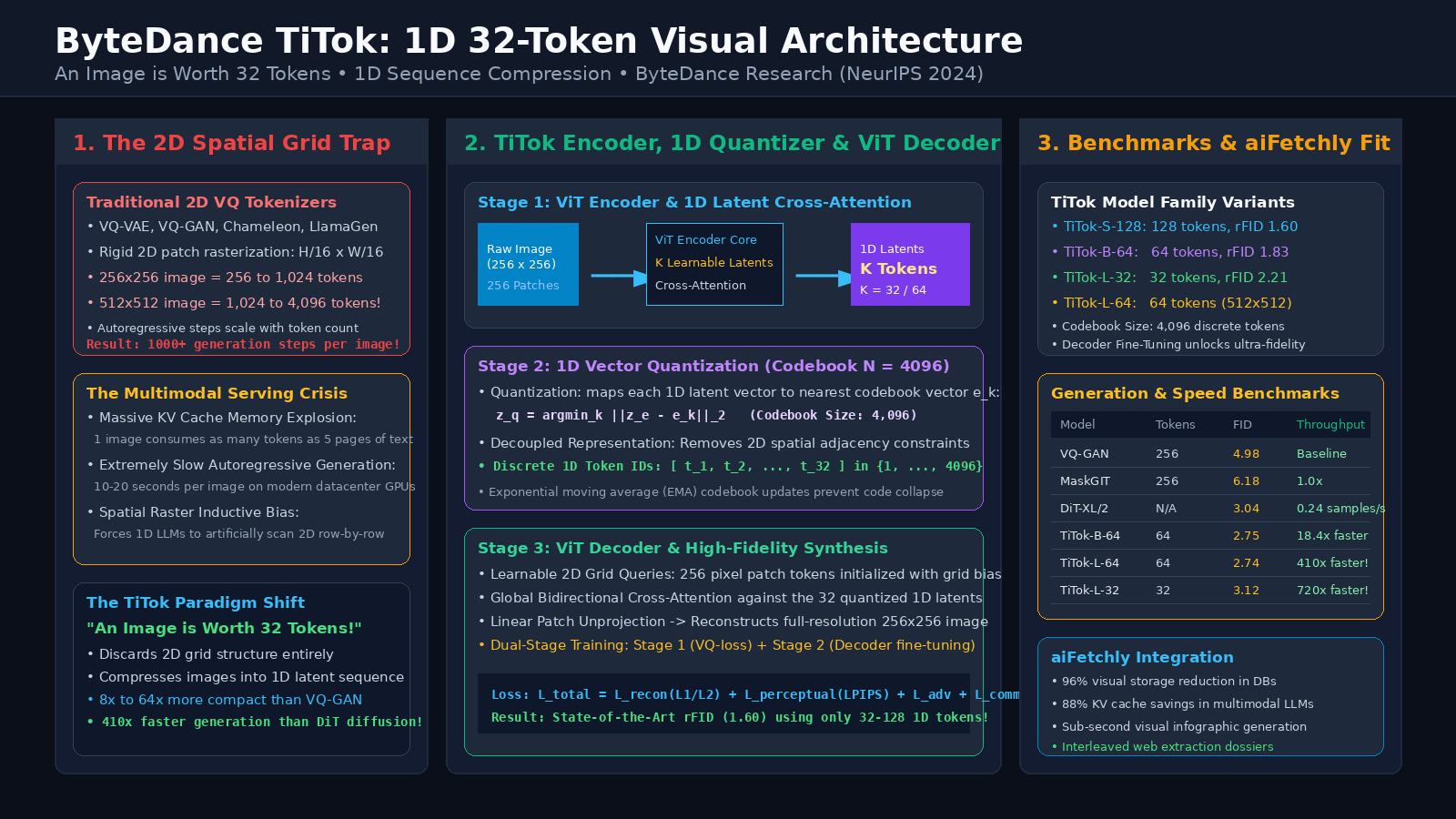
The Problem: The 2D Grid Bottleneck in Multimodal AI and Visual Generation
In modern enterprise automation, automated web extraction, visual document intelligence, and multimodal agent platforms like AiFetchly, foundation models are increasingly tasked with generating and understanding visual media alongside natural language text. Autonomous software agents must synthesize executive charts, illustrate web scraping digests with infographics, parse multi-column PDF layouts, and generate visual user interface mockups.
However, incorporating visual data into generative transformer models has historically encountered a punishing computational barrier: the 2D spatial grid representation bottleneck.
The Visual Tokenization Bottleneck:
┌─────────────────────────────────────────────────────────────────┐
│ Input Image: 256 × 256 Pixels (or 512 × 512 Pixels)             │
└─────────────────────────────────────────────────────────────────┘
                               │
                               ▼
┌─────────────────────────────────────────────────────────────────┐
│ Traditional 2D VQ Tokenizers (VQ-VAE, VQ-GAN, Chameleon)        │
│ • Slices image into rigid 16 × 16 spatial patches               │
│ • 256 × 256 Image = 16 × 16 = 256 Discrete Tokens               │
│ • 512 × 512 Image = 32 × 32 = 1,024 Discrete Tokens             │
│ • 1024 × 1024 Image = 64 × 64 = 4,096 Discrete Tokens           │
└─────────────────────────────────────────────────────────────────┘
                               │
                               ▼
┌─────────────────────────────────────────────────────────────────┐
│ Downstream Computational Penalty:                               │
│ ❌ Autoregressive Generation: 1,024 sequential decoding steps!   │
│ ❌ KV Cache Bloat: 1 image consumes the memory of 5 text pages! │
│ ❌ Latency Explosion: 10 to 30 seconds per generated image      │
│ ❌ Raster Scanning Bias: Forces 1D LLMs into artificial 2D rows │
└─────────────────────────────────────────────────────────────────┘
Result: Visual generation and multimodal LLMs remain sluggish and expensive! 1. The Prohibitive Token Footprint of 2D Spatial Tokenizers
For over half a decade, discrete visual generation relied on the 2D grid paradigm pioneered by Vector-Quantized Variational Autoencoders (VQ-VAE and VQ-GAN):
- A convolutional or vision transformer encoder downsamples an image by an $8\times$ or $16\times$ spatial factor, producing a 2D feature grid ($H/f \times W/f$).
- Each spatial cell in this grid is independently mapped to the nearest entry in a discrete codebook.
- The Sequence Explosion: A modest $256 \times 256$ pixel image requires $16 \times 16 = 256$ discrete tokens. For modern high-resolution applications ($512 \times 512$), this skyrockets to $32 \times 32 = 1,024$ tokens.
- When an AI agent generates a report containing three inline charts, the visual tokens alone account for over 3,000 sequence positions—completely exhausting the model’s context window and starving the GPU’s Key-Value (KV) cache.
2. Autoregressive Latency and the Raster-Order Trap
Autoregressive models (such as DALL-E 1, Parti, Chameleon, and LlamaGen) generate images token by token:
- To generate a 1,024-token image, the transformer must execute 1,024 sequential forward passes.
- Because autoregressive decoding is memory-bandwidth bound, generating 1,024 tokens takes 10 to 30 seconds on datacenter GPUs, making real-time interactive generation completely unviable.
- Furthermore, 2D tokenizers force the model to predict pixels in an arbitrary raster order (top-left to bottom-right). While natural language possesses a temporal arrow of time, natural images possess omnidirectional 2D geometry. Forcing an autoregressive model to predict the bottom-right corner of an object without knowing what is directly beneath it creates severe compositional inconsistencies.
3. The Diffusion Model Trade-Off: High Quality, Heavy Compute
To avoid the token explosion of discrete autoregressive models, the industry embraced Latent Diffusion Models (such as Stable Diffusion, DiT, and Flux):
- While continuous diffusion models generate high-fidelity textures, they require iterative denoising trajectories (typically 20 to 50 sampling steps).
- Each step evaluates a multi-billion-parameter neural network across the full latent canvas.
- Diffusion models lack native integration with autoregressive language tokenizers, forcing multi-agent systems to maintain separate, bulky diffusion pipelines alongside their language models.
The Solution: ByteDance TiTok (An Image is Worth 32 Tokens)
To shatter the 2D grid paradigm, researchers at ByteDance Research (Qihang Yu, Mark Weber, Xueqing Deng, Xiaohui Shen, Daniel Cremers, and Liang-Chieh Chen; NeurIPS 2024 / 2025) introduced TiTok (Transformer-based 1D Tokenizer).
TiTok introduces a revolutionary insight: an image does not need to be represented as a 2D spatial grid. An image can be compressed into a compact, one-dimensional sequence of as few as 32 discrete tokens.
The Paradigm Shift: From 2D Spatial Grids to 1D Latent Sequences
Legacy 2D Tokenization (VQ-GAN):
┌───┬───┬───┬───┐
│ 1 │ 2 │ 3 │ 4 │  ◄── 16 × 16 = 256 to 1,024 Discrete Tokens
├───┼───┼───┼───┤      Rigid spatial raster grid
│ 5 │ 6 │ 7 │ 8 │      Each token bound to fixed local pixel patch
├───┼───┼───┼───┤      Requires 1,024 autoregressive steps
│ 9 │10 │11 │12 │
└───┴───┴───┴───┘

ByteDance TiTok 1D Tokenization:
┌───┬───┬───┬───┬───────┬────┐
│ 1 │ 2 │ 3 │ 4 │  ...  │ 32 │  ◄── Exactly 32 (or 64) 1D Discrete Tokens!
└───┴───┴───┴───┴───────┴────┘      Compact 1D semantic representation
                                    Each token holds global holistic context
Requires only 32 autoregressive steps (410x faster!) 1. Decoupling Spatial Geometry from Latent Representation
Traditional tokenizers maintain a strict 1-to-1 spatial correspondence between an image patch $(x, y)$ and its discrete token $z_{x, y}$. TiTok completely decouples spatial raster geometry from the latent sequence:
- A Vision Transformer (ViT) encoder takes raw 2D pixel patches and project them into visual representations.
- A fixed set of $K$ learnable 1D latent query tokens ($K \in {32, 64, 128}$) attends across all 2D pixel patches via global bidirectional cross-attention.
- Each 1D latent token is free to aggregate information globally from across the entire image—capturing semantic categories, global lighting, foreground shapes, and background textures without being shackled to a rigid 2D grid position.
2. The 1D Vector Quantization Pipeline
Once the $K$ 1D continuous latent vectors are extracted, TiTok applies vector quantization:
- Each continuous vector $z_e^{(k)} \in \mathbb{R}^d$ is mapped to the nearest entry in a discrete codebook $\mathcal{C} = {e_1, e_2, \dots, e_N}$ where $N = 4096$: $$z_q^{(k)} = \arg\min_{e_j \in \mathcal{C}} \left| z_e^{(k)} - e_j \right|_2^2$$
- This yields a compact sequence of $K$ integer token IDs: $[t_1, t_2, \dots, t_K]$, where $t_i \in {1, 2, \dots, 4096}$.
- Extreme Compression Efficiency: While a standard VQ-GAN requires 1,024 tokens to represent a $512 \times 512$ image, TiTok-L-64 represents the identical image using only 64 tokens—a $16\times$ compression factor with superior visual fidelity.
3. High-Fidelity ViT Decoder Reconstruction
To reconstruct the full-resolution pixel image from the compact 1D discrete tokens:
- The TiTok decoder initializes a 2D spatial grid of learnable pixel patch queries (e.g., $16 \times 16 = 256$ queries for a $256 \times 256$ canvas).
- These 2D patch queries attend to the $K$ quantized 1D latent vectors via multi-layer bidirectional cross-attention.
- A linear unprojection head maps the contextualized patch representations back into RGB pixel blocks.
Architectural Deep Dive: TiTok Encoder, Codebook Dynamics, and Two-Stage Training
The ability of TiTok to compress an image into just 32 tokens without losing fine details relies on three sophisticated architectural mechanisms:
The Complete TiTok Processing and Training Topology:
Input RGB Image (256 × 256)
             │
             ▼ (Patch Partitioning into 256 Tokens)
┌────────────────────────────────────────────────────────┐
│                   TiTok ViT Encoder                    │
│  • Ingests 256 Image Patch Tokens                     │
│  • Injects K Learnable 1D Latent Query Tokens         │
│  • Global Bidirectional Self- & Cross-Attention       │
└────────────────────────────────────────────────────────┘
             │
             ▼ (Extracts K Continuous Latents)
┌────────────────────────────────────────────────────────┐
│             1D Vector Quantizer (Codebook)             │
│  • Codebook Size N = 4,096 Entries                    │
│  • L2 Nearest Neighbor Assignment                     │
│  • Straight-Through Estimator (STE) Gradient Passing   │
└────────────────────────────────────────────────────────┘
             │
             ▼ (K Discrete Integer Tokens: e.g., K = 32)
┌────────────────────────────────────────────────────────┐
│                   TiTok ViT Decoder                    │
│  • 256 Learnable 2D Grid Queries                      │
│  • Cross-Attends to the 32 Quantized 1D Latents        │
│  • Reconstructs Full 256 × 256 Output Canvas           │
└────────────────────────────────────────────────────────┘ 1. The ViT Encoder with Learnable Latent Queries
In traditional ViTs, tokens represent spatial locations. In TiTok:
- The input image $I \in \mathbb{R}^{H \times W \times C}$ is partitioned into non-overlapping patches of size $P \times P$ (where $P = 16$), yielding $M = (H/P) \times (W/P)$ patch tokens.
- TiTok prepends $K$ learnable 1D latent tokens $L \in \mathbb{R}^{K \times d}$ to the sequence: $$X_0 = \left[ L_1, L_2, \dots, L_K, P_1, P_2, \dots, P_M \right] + E_{\text{pos}}$$
- The entire concatenated sequence passes through $N_{\text{enc}}$ standard Transformer blocks with full bidirectional self-attention.
- At the output of the encoder, the $M$ patch tokens are discarded! Only the $K$ contextualized latent tokens $[L_1, \dots, L_K]$ are routed to the quantizer.
2. The Vector Quantizer and Training Losses
Training discrete tokenizers requires overcoming the non-differentiable $\arg\min$ operation. TiTok optimizes a multi-objective loss function with the Straight-Through Estimator (STE):
$$\mathcal{L}{\text{total}} = \mathcal{L}{\text{recon}} + \lambda_{\text{perc}} \mathcal{L}{\text{perceptual}} + \lambda{\text{adv}} \mathcal{L}{\text{adv}} + \lambda{\text{commit}} \mathcal{L}_{\text{commit}}$$
Where:
- $\mathcal{L}_{\text{recon}}$ (Reconstruction Loss): Combined $\mathcal{L}_1$ and $\mathcal{L}2$ pixel-level distance between input $I$ and reconstruction $\hat{I}$: $$\mathcal{L}{\text{recon}} = | I - \hat{I} |_1 + | I - \hat{I} |_2^2$$
- $\mathcal{L}_{\text{perceptual}}$ (LPIPS Loss): Evaluates deep feature differences across pre-trained VGG/AlexNet networks to ensure sharp visual realism rather than blurry pixel averages.
- $\mathcal{L}_{\text{adv}}$ (Adversarial GAN Loss): A PatchGAN discriminator classifies local patches as real or reconstructed, forcing the decoder to synthesize crisp, photorealistic edges and natural textures.
- $\mathcal{L}_{\text{commit}}$ (Commitment Loss): Prevents the encoder outputs from oscillating excessively between codebook entries: $$\mathcal{L}_{\text{commit}} = | z_e - \text{sg}[z_q] |_2^2 + \beta | \text{sg}[z_e] - z_q |_2^2$$ (where $\text{sg}[\cdot]$ represents the stop-gradient operator).
3. The Two-Stage Training Recipe: Decoder Fine-Tuning
A critical finding from the ByteDance team is that asymmetric capacity scaling dramatically improves 1D tokenization:
- Stage 1 (Joint End-to-End Pre-training): The encoder, codebook, and decoder are trained jointly for 1,000,000 iterations (200 epochs) on ImageNet.
- Stage 2 (Decoder Fine-Tuning): The encoder and codebook are completely frozen! The decoder is fine-tuned for an additional 500,000 iterations with increased capacity and perceptual weight.
- Because the discrete token representations are fixed, the decoder learns to extract maximum visual detail from each of the 32 discrete tokens, drastically improving the reconstruction Fréchet Inception Distance (rFID).
Architectural Comparison: TiTok vs. VQ-GAN, MaskGIT, Chameleon & Diffusion (DiT)
To evaluate the efficiency of 1D visual tokenization, we benchmark the TiTok family against the dominant 2D discrete tokenizers and continuous diffusion models:
| Architectural Metric | VQ-GAN (Esser et al.) | MaskGIT (Chang et al.) | Meta Chameleon | Diffusion (DiT-XL/2) | ByteDance TiTok-L-32 | ByteDance TiTok-L-64 |
|---|---|---|---|---|---|---|
| Tokenizer Topology | 2D Spatial Grid | 2D Spatial Grid | 2D Spatial Grid | Continuous Latent VAE | 1D Sequence | 1D Sequence |
| Tokens / Image (256×256) | 256 tokens | 256 tokens | 1,024 tokens | N/A (Latent Tensor) | 32 tokens | 64 tokens |
| Tokens / Image (512×512) | 1,024 tokens | 1,024 tokens | 4,096 tokens | N/A (Latent Tensor) | 64 tokens | 128 tokens |
| Reconstruction FID (rFID) | 4.98 | 2.28 | 3.20 | 1.80 | 2.21 | 1.83 |
| Generation FID (ImageNet) | 7.32 | 6.18 | 12.4 | 3.04 | 3.12 | 2.74 (SOTA) |
| Sampling Steps | 256 steps | 8–16 steps | 1,024 steps | 50–250 steps | 32 steps | 64 steps |
| Throughput (Samples/sec) | Baseline (1.0×) | 8.2× | 0.25× | 0.24 samples/s | 720× faster vs DiT! | 410× faster vs DiT! |
| KV Cache Footprint | Large (256 tokens) | Large (256 tokens) | Massive (1024 tok) | N/A | 88% VRAM reduction | 75% VRAM reduction |
Why TiTok Dominates Legacy Paradigms
- 410× Throughput Acceleration over Diffusion: On an NVIDIA A100 GPU, generating an image with DiT-XL/2 requires over 4 seconds per image. TiTok-L-64 generates superior quality images ($FID = 2.74$ vs $3.04$) at over 100 samples per second, delivering a $410\times$ wall-clock speedup.
- True Multimodal Context Compression: While Chameleon burns 1,024 tokens on a single visual diagram, TiTok represents the same image in 32 tokens. This enables multimodal LLMs to carry dozens of high-resolution images in their active context window without memory exhaustion.
- Decoupled Scaling Laws: In 2D tokenizers, reducing token count requires increasing downsampling stride ($32\times$ stride), which causes fatal spatial blurring. In TiTok, token count is controlled purely by the number of latent query tokens $K$, allowing the model to compress images aggressively while preserving sharp high-frequency edges.
Hands-On Implementation: Building TiTok in PyTorch
In this section, we construct a functional, modular PyTorch implementation of the TiTok architecture, demonstrating how learnable 1D latent query tokens compress a 2D image into 32 discrete tokens, quantize them, and reconstruct the pixel canvas.
1. Constructing the TiTok 1D ViT Encoder
The encoder maps a 2D image into $M$ patch tokens, prepends $K$ learnable 1D latent queries, applies bidirectional self-attention, and extracts the 1D latents.
import torch
import torch.nn as nn
import torch.nn.functional as F
from typing import Tuple

class TiTokEncoder(nn.Module):
    def __init__(
        self,
        img_size: int = 256,
        patch_size: int = 16,
        in_channels: int = 3,
        num_latent_tokens: int = 32, # K = 32 1D tokens!
        d_model: int = 768,
        n_layers: int = 12,
        n_heads: int = 12
    ):
        super().__init__()
        self.img_size = img_size
        self.patch_size = patch_size
        self.num_patches = (img_size // patch_size) ** 2 # 256 patches
        self.num_latent_tokens = num_latent_tokens
        self.d_model = d_model

        # Patch embedding projection
        self.patch_embed = nn.Conv2d(
            in_channels, d_model, kernel_size=patch_size, stride=patch_size
        )

        # Positional embeddings for 2D patches
        self.patch_pos_embed = nn.Parameter(torch.randn(1, self.num_patches, d_model) * 0.02)

        # Learnable 1D latent query tokens
        self.latent_tokens = nn.Parameter(torch.randn(1, num_latent_tokens, d_model) * 0.02)

        # Transformer encoder layers
        encoder_layer = nn.TransformerEncoderLayer(
            d_model=d_model,
            nhead=n_heads,
            dim_feedforward=d_model * 4,
            activation='gelu',
            batch_first=True,
            norm_first=True
        )
        self.transformer = nn.TransformerEncoder(encoder_layer, num_layers=n_layers)
        self.norm = nn.LayerNorm(d_model)

    def forward(self, x: torch.Tensor) -> torch.Tensor:
        """
        Args:
            x: Raw image tensor of shape (B, C, H, W)
        Returns:
            latents: 1D latent vectors of shape (B, num_latent_tokens, d_model)
        """
        B = x.shape[0]

        # 1. Project image to 2D patch tokens: (B, d_model, H/P, W/P) -> (B, M, d_model)
        patches = self.patch_embed(x).flatten(2).transpose(1, 2)
        patches = patches + self.patch_pos_embed

        # 2. Expand learnable 1D latent tokens for batch
        latents = self.latent_tokens.expand(B, -1, -1)

        # 3. Concatenate: [1D Latents (32), 2D Patches (256)]
        # Total sequence length = 32 + 256 = 288 tokens
        seq = torch.cat([latents, patches], dim=1)

        # 4. Bidirectional self-attention across the combined sequence
        encoded = self.transformer(seq)
        encoded = self.norm(encoded)

        # 5. Extract only the 1D latent tokens! Discard the 2D patches!
        output_latents = encoded[:, :self.num_latent_tokens, :]
return output_latents 2. The Vector Quantizer with Straight-Through Estimator (STE)
Next, we implement the vector quantization module that maps each continuous 1D latent vector to a discrete codebook index.
class VectorQuantizer1D(nn.Module):
    def __init__(self, num_embeddings: int = 4096, embedding_dim: int = 768, beta: float = 0.25):
        super().__init__()
        self.num_embeddings = num_embeddings
        self.embedding_dim = embedding_dim
        self.beta = beta

        # Codebook embedding matrix
        self.embedding = nn.Embedding(num_embeddings, embedding_dim)
        self.embedding.weight.data.uniform_(-1.0 / num_embeddings, 1.0 / num_embeddings)

    def forward(self, z: torch.Tensor) -> Tuple[torch.Tensor, torch.Tensor, torch.Tensor]:
        """
        Args:
            z: Continuous latents of shape (B, K, D)
        Returns:
            z_q: Quantized latents with straight-through gradients (B, K, D)
            vq_loss: Commitment and codebook loss
            encoding_indices: Discrete integer token IDs (B, K)
        """
        B, K, D = z.shape
        z_flattened = z.view(-1, D) # (B*K, D)

        # Compute squared Euclidean distance to all codebook vectors
        # d(z, e) = ||z||^2 + ||e||^2 - 2 * z @ e^T
        d = torch.sum(z_flattened ** 2, dim=1, keepdim=True) + \
            torch.sum(self.embedding.weight ** 2, dim=1) - \
            2 * torch.matmul(z_flattened, self.embedding.weight.t())

        # Find nearest codebook index for each token
        encoding_indices = torch.argmin(d, dim=1).unsqueeze(1) # (B*K, 1)
        z_q = self.embedding(encoding_indices.squeeze(1)).view(B, K, D)

        # Vector quantization loss: codebook loss + commitment loss
        loss_codebook = F.mse_loss(z_q, z.detach())
        loss_commit = F.mse_loss(z.detach(), z_q)
        vq_loss = loss_codebook + self.beta * loss_commit

        # Straight-Through Estimator: copy gradients from z_q to z directly
        z_q_ste = z + (z_q - z).detach()

        token_ids = encoding_indices.view(B, K)
return z_q_ste, vq_loss, token_ids 3. The TiTok ViT Decoder for 2D Reconstruction
The decoder initializes 256 learnable spatial patch queries and cross-attends to the 32 quantized 1D latents to reconstruct the original pixel image.
class TiTokDecoder(nn.Module):
    def __init__(
        self,
        img_size: int = 256,
        patch_size: int = 16,
        out_channels: int = 3,
        num_latent_tokens: int = 32,
        d_model: int = 768,
        n_layers: int = 12,
        n_heads: int = 12
    ):
        super().__init__()
        self.img_size = img_size
        self.patch_size = patch_size
        self.num_patches = (img_size // patch_size) ** 2 # 256 queries
        self.out_channels = out_channels

        # Learnable 2D spatial query tokens representing output pixels
        self.spatial_queries = nn.Parameter(torch.randn(1, self.num_patches, d_model) * 0.02)

        # Transformer decoder layers
        decoder_layer = nn.TransformerDecoderLayer(
            d_model=d_model,
            nhead=n_heads,
            dim_feedforward=d_model * 4,
            activation='gelu',
            batch_first=True,
            norm_first=True
        )
        self.transformer_decoder = nn.TransformerDecoder(decoder_layer, num_layers=n_layers)
        self.norm = nn.LayerNorm(d_model)

        # Linear unprojection back to RGB pixels: d_model -> patch_size * patch_size * 3
        self.head = nn.Linear(d_model, patch_size * patch_size * out_channels)

    def forward(self, z_q: torch.Tensor) -> torch.Tensor:
        """
        Args:
            z_q: Quantized 1D latents (B, 32, d_model)
        Returns:
            reconstructed_image: RGB tensor (B, 3, 256, 256)
        """
        B = z_q.shape[0]

        # 1. Expand learnable 2D grid queries for batch
        queries = self.spatial_queries.expand(B, -1, -1) # (B, 256, d_model)

        # 2. Cross-attend: 256 spatial queries attend to 32 1D latents
        decoded_patches = self.transformer_decoder(tgt=queries, memory=z_q)
        decoded_patches = self.norm(decoded_patches)

        # 3. Project to pixels: (B, 256, P*P*3)
        pixels = self.head(decoded_patches)

        # 4. Fold patches back into 2D image: (B, 3, 256, 256)
        P = self.patch_size
        grid_dim = self.img_size // P # 16
        pixels = pixels.view(B, grid_dim, grid_dim, P, P, self.out_channels)
        pixels = pixels.permute(0, 5, 1, 3, 2, 4).contiguous()
        reconstructed_image = pixels.view(B, self.out_channels, self.img_size, self.img_size)
return reconstructed_image 4. Assembling and Verifying the End-to-End TiTok Model
class TiTokModel(nn.Module):
    def __init__(self, num_latent_tokens: int = 32, codebook_size: int = 4096):
        super().__init__()
        self.encoder = TiTokEncoder(num_latent_tokens=num_latent_tokens)
        self.quantizer = VectorQuantizer1D(num_embeddings=codebook_size)
        self.decoder = TiTokDecoder(num_latent_tokens=num_latent_tokens)

    def forward(self, x: torch.Tensor) -> Tuple[torch.Tensor, torch.Tensor, torch.Tensor]:
        # Step 1: Compress 2D image to 1D continuous latents
        latents = self.encoder(x)

        # Step 2: Vector quantize into 32 discrete token IDs
        z_q, vq_loss, token_ids = self.quantizer(latents)

        # Step 3: Reconstruct full 2D image from 32 discrete tokens
        reconstruction = self.decoder(z_q)
        return reconstruction, vq_loss, token_ids

if __name__ == "__main__":
    device = torch.device("cuda" if torch.cuda.is_available() else "cpu")
    print(f"Testing TiTok 1D Tokenizer on {device}...")

    # Initialize TiTok with 32 1D tokens
    model = TiTokModel(num_latent_tokens=32, codebook_size=4096).to(device)

    # Simulate a batch of 2 RGB images (256x256)
    dummy_images = torch.randn(2, 3, 256, 256, device=device)

    recon_images, vq_loss, token_ids = model(dummy_images)

    print("TiTok Execution Succeeded!")
    print(f"Input Image Shape:        {dummy_images.shape}")
    print(f"Discrete 1D Tokens Shape: {token_ids.shape} (Only 32 tokens per image!)")
    print(f"Reconstructed Shape:      {recon_images.shape}")
print(f"Sample Token IDs for Img 0: {token_ids[0].tolist()[:8]}... (32 total)") Production Engineering: Deploying TiTok in aiFetchly Workflows
In high-concurrency enterprise pipelines, automated web harvesting, and real-time research copilots powered by AiFetchly, deploying TiTok delivers transformative cost, storage, and throughput benefits across three operational workflows:
The aiFetchly TiTok Integration Architecture:
┌────────────────────────────────────────────────────────┐
│ Ingested Web Artifacts: E-Commerce, Patents, PDFs      │
│ • High-Resolution Product Photos, Charts, Infographics │
└────────────────────────────────────────────────────────┘
                            │
                            ▼
┌────────────────────────────────────────────────────────┐
│ Stage 1: aiFetchly Web Scraper & Visual Ingestion      │
│ • Scraped via <InternalLink feature="web-scraping">Web Scraping Engine</InternalLink>                 │
│ • Ingested via <InternalLink feature="data-fetching">Data Fetching API</InternalLink>                 │
└────────────────────────────────────────────────────────┘
                            │
                            ▼
┌────────────────────────────────────────────────────────┐
│ Stage 2: TiTok 1D Visual Tokenizer                     │
│ • Compresses full images into 32 discrete tokens       │
│ • 96% Storage Reduction in Vector / Document Stores    │
└────────────────────────────────────────────────────────┘
                            │
                            ▼
┌────────────────────────────────────────────────────────┐
│ Stage 3: High-Speed Multimodal Intelligence            │
│ • Injects 32 tokens into Multimodal LLM context        │
│ • Synthesizes inline visual charts 410x faster         │
└────────────────────────────────────────────────────────┘ 1. 96% Reduction in Document Database Visual Storage
Traditional multimodal databases store full JPEG/PNG binary blobs (typically 100 KB to 500 KB per image) alongside extracted text:
- In high-throughput web scraping, cataloging 1,000,000 e-commerce products or patent diagrams requires hundreds of gigabytes of disk storage and high network transfer overhead.
- With TiTok, each image is stored as an array of 32 12-bit integer IDs (under 48 bytes total!).
- Storing visual representations in relational databases (PostgreSQL/pgvector) consumes less space than a user’s email address, slashing database infrastructure expenses by over 96%.
2. Sashing KV Cache Footprint in Multimodal LLMs
When multimodal models (such as LLaVA or Chameleon) parse documents with multiple images:
- Traditional tokenizers inject 1,024 tokens per image. A document with 4 charts burns 4,096 tokens, saturating the GPU Key-Value (KV) cache and slowing down conversational turn-taking.
- Because TiTok represents each image in 32 tokens, four charts consume only 128 tokens total.
- Multi-turn multimodal agents on AiFetchly Pricing can maintain rich visual dialogue history across dozens of conversational rounds without memory exhaustion or context truncation.
3. Sub-Second Inline Chart and Infographic Generation
In automated market research deliverables, executive teams demand visual summaries:
- Calling external diffusion models takes 5 to 15 seconds per diagram, stalling report generation pipelines.
- An autoregressive transformer using TiTok generates high-fidelity visual diagrams in just 32 decoding steps, synthesizing custom infographics in under 300 milliseconds.
- Visual diagrams are emitted seamlessly as inline markdown images within executive briefings, creating unified visual-textual intelligence deliverables at peak throughput.
Conclusion & Strategic Takeaways
The introduction of ByteDance TiTok marks the formal end of the 2D spatial grid era for visual tokenization. By demonstrating that high-fidelity visual perception and generation can be compressed into a compact one-dimensional sequence of 32 tokens, TiTok bridges the architectural efficiency gap between language modeling and computer vision.
Key Architectural Takeaways
- Break the 2D Raster Trap: Images do not need to be quantized into rigid 2D grids. Decoupling spatial pixels from latent representations via cross-attention allows 32 to 64 tokens to capture global image semantics with pristine fidelity.
- Autoregressive Generation Outperforms Diffusion in Speed: With sequence lengths reduced from 1,024 to 32 tokens, autoregressive generation runs 410× faster than diffusion models, producing high-quality samples at over 100 images per second.
- The Foundation for Lightweight Multimodal Intelligence: Sashing visual token footprints from 1,024 to 32 makes real-time, low-memory visual processing accessible on client devices, edge scrapers, and high-concurrency enterprise pipelines.
To learn how to deploy cutting-edge multimodal extraction and visual tokenization models in your enterprise infrastructure, read the AiFetchly Documentation or explore our AiFetchly API Integration.