TabPFN Guide: Tabular Foundation Models & In-Context AI

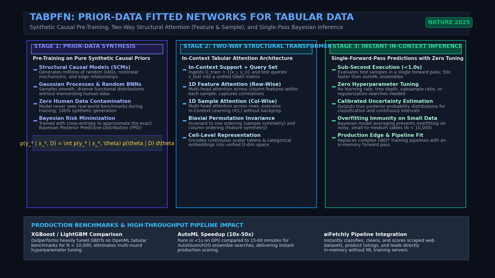
The Problem: The GBDT Bottleneck in Modern Agentic AI & Data Pipelines

In modern enterprise automation, automated market intelligence, and continuous web data extraction platforms powered by AiFetchly, data ingestion is fundamentally tabular. When automated web workers scrape competitor product catalogs, extract financial 10-K balance sheets, harvest real-time commercial real estate registries, or compile prospective sales leads, the resulting payloads land as structured tables with rows of heterogeneous entities and columns of numeric, categorical, and text attributes.

To transform this harvested raw tabular data into actionable business value, software architectures require immediate predictive modeling:

• Classifying incoming leads as high-intent vs. low-intent.
• Predicting market clearing prices or financial default probabilities.
• Imputing missing attributes in harvested e-commerce catalogs.
• Detecting fraudulent anomalies in real-time transaction tables.

However, while natural language processing and computer vision have completely transitioned to pre-trained foundation models that execute zero-shot or in-context predictions instantaneously, tabular machine learning has remained stubbornly trapped in the manual Gradient Boosted Decision Tree (GBDT) paradigm.

1. The Iterative Fitting Tax and Hyperparameter Grid Search Wall

For over a decade, algorithms like XGBoost, LightGBM, and CatBoost have represented the gold standard for tabular data. However, their operational mechanics are fundamentally incompatible with real-time, autonomous AI systems:

• Sequential Iterative Fitting: GBDTs build an ensemble of shallow decision trees sequentially. Each tree fits the residual errors of preceding trees. This means training cannot be evaluated in a single parallel matrix multiplication; it requires thousands of sequential tree splits across CPU memory.
• The Hyperparameter Sensitivity Curse: Unlike foundation models that generalize out-of-the-box, the accuracy of a GBDT is acutely sensitive to hyperparameter configurations. A default XGBoost model with max_depth=6 and learning_rate=0.3 frequently overfits catastrophically on small or noisy datasets.
• Automated Machine Learning (AutoML) Latency: To counteract hyperparameter sensitivity, production pipelines deploy AutoML wrappers (such as AutoGluon, FLAML, or H2O). These engines train dozens of gradient boosted trees, neural networks, and stacking ensembles across multiple cross-validation folds. A single dataset with 2,000 rows can take 10 to 60 minutes of intense CPU thrashing to find an optimal ensemble. For an autonomous AI agent executing live data harvesting, waiting an hour to make a single prediction breaks the operational loop completely.

2. The Overfitting Crisis on Small-to-Medium Tabular Datasets

In production web scraping and enterprise analytics, datasets are rarely composed of millions of rows. High-value data is frequently constrained to small-to-medium horizons:

• 500 rows of competitive pricing from a niche industrial supplier.
• 1,200 labeled contracts in an enterprise legal review.
• 3,000 patient records in a clinical trial study.

On datasets with fewer than $10,000$ rows ($N < 10,000$), traditional parametric models and GBDTs suffer from severe variance and overfitting:

• Heuristic Greedy Splits: Tree building relies on greedy heuristics (such as Gini impurity or variance reduction) calculated at individual leaf nodes. On small sample sizes, random statistical noise causes the algorithm to create spurious branch splits that fail on unseen out-of-sample data.
• Under-Calibrated Probabilities: When an overfitted decision tree isolates three training samples in a leaf, it outputs a predicted probability of $1.0$ (100% confidence). In downstream agentic workflows where decisions trigger automated emails, financial trades, or database updates, uncalibrated overconfident probabilities lead to disastrous automated actions.

3. The Structural Disconnect: Why Trees Cannot Learn In-Context

Language models like GPT-4o, Claude 3.5 Sonnet, and DeepSeek-V3 demonstrate remarkable In-Context Learning (ICL): you provide three examples of a formatting task inside the prompt, and the model immediately performs the task on a fourth example without modifying its parameter weights.

GBDTs cannot perform In-Context Learning:

• They maintain no internal memory of prior datasets. Every new table is an isolated, tabula rasa event.
• An XGBoost model trained on yesterday’s scraped housing data cannot leverage its learned structural knowledge when evaluating today’s commercial real estate listings; it must be trained from scratch.
• Software engineers are forced to maintain complex, brittle MLOps infrastructure: database tables for training data, cron jobs for periodic retraining, model registries for storing pickled artifact weights, and dedicated microservice inference containers.

To eliminate this operational tax, the machine learning research community sought a holy grail: a pre-trained foundation model that ingests an entire tabular dataset as context and outputs exact, optimal predictions in a single forward pass.

The Solution: Prior-Data Fitted Networks & Bayesian Posterior Estimation

Published in Nature (January 2025) by researchers from Prior Labs and the University of Freiburg (Noah Hollmann, Samuel Müller, Katharina Eggensperger, and Frank Hutter), TabPFN (Prior-Data Fitted Networks for Tabular Data) represents the first true foundation model for tabular data.

Instead of fitting decision trees on the fly, TabPFN reframes tabular machine learning as an in-context approximation of exact Bayesian inference.

1. Mathematical Formulation: Approximating the Bayesian Posterior Predictive Distribution

In classical statistics and Bayesian probability theory, the theoretically optimal method for making predictions from data is Bayesian Model Averaging (BMA).

Suppose nature generates datasets using a parameterized data-generating mechanism $ heta$ drawn from a universal prior over functions $p(\theta)$. Given an observed training dataset $D = &#123;(x_1, y_1), (x_2, y_2), \dots, (x_n, y_n)&#125;$ and an unlabelled test query $x_*$, the Bayesian Posterior Predictive Distribution (PPD) is defined as:

$$p(y_* \mid x_, D) = \int p(y_ \mid x_*, \theta) , p(\theta \mid D) , d\theta$$

Where $p(\theta \mid D)$ is the posterior distribution over the parameters:

$$p(\theta \mid D) = \frac{p(D \mid \theta) , p(\theta)}{\int p(D \mid \theta’) , p(\theta’) , d\theta’}$$

The PPD integrates over every conceivable model, decision boundary, and parameter setting weighted by how well it explains the observed data $D$.

Historically, calculating this integral was computationally impossible for real-world tables because the parameter space $\Theta$ is infinite and high-dimensional, requiring intractable Markov Chain Monte Carlo (MCMC) sampling.

The Fundamental Insight of Prior-Data Fitted Networks (PFNs): A neural network with parameters $\mathbf{w}$ can be trained to directly approximate the Posterior Predictive Distribution $p(y_* \mid x_*, D)$ across an infinite family of datasets by minimizing the cross-entropy loss over synthetic datasets sampled from a rich prior $p(D)$:

$$ \mathcal{L}(\mathbf{w}) = - \mathbb{E}{D \sim p(D), (x, y_) \sim D} \left[ \log q_{\mathbf{w}}(y_* \mid x_*, D) ight] $$

Müller et al. (2022) mathematically proved that when a Transformer $q_{\mathbf{w}}$ is optimized with cross-entropy loss over datasets drawn from prior $p(D)$, the global minimizer of the loss function is identically equal to the true Bayesian Posterior Predictive Distribution:

$$\arg\min_{\mathbf{w}} \mathcal{L}(\mathbf{w}) \equiv p(y_* \mid x_*, D)$$

By training once on millions of synthetic priors, TabPFN distills the intractable Bayesian integral into the feedforward weights of a single Transformer. At inference time, calculating the optimal Bayesian prediction requires only a single forward pass.

2. Synthetic Pre-Training on Causal Graphs & Gaussian Processes

A foundational question arises: Where did Prior Labs acquire the training data to teach TabPFN how to predict tabular tables?

If a model is trained on scraped real-world tables (like OpenML or Kaggle), it risks data leakage, privacy violations, and overfitting to specific domains.

TabPFN takes a radically different path: it is trained exclusively on 100% synthetically generated data.

During its extensive pre-training phase:

• TabPFN ingested millions of uniquely generated synthetic datasets.
• Each synthetic dataset had a randomly chosen number of features ($d \le 500$), a random number of samples ($n \le 10,000$), random noise levels, varying class balances, and diverse non-linear correlations.
• The model never memorized human facts; it learned the universal structural geometry of tabular dependencies.
• Because it has never seen a real-world table during training, it is physically impossible for TabPFN to memorize or leak sensitive enterprise data.

3. In-Context Learning for Tabular Data

In natural language processing, LLMs process a sequence of text tokens:

$$ ext{“The capital of France is”} \longrightarrow ext{“Paris”}$$

In TabPFN, the context consists of entire tabular rows. The training dataset $D_{\text{train}} = &#123;(x_1, y_1), \dots, (x_n, y_n)&#125;$ acts as the few-shot context support set, and the test rows $X_{\text{test}} = &#123;x_{n+1}, \dots, x_{n+m}&#125;$ act as the unlabeled query tokens:

$$[(x_1, y_1), (x_2, y_2), \dots, (x_n, y_n), (x_{n+1}, ?)] \longrightarrow p(y_{n+1})$$

When you pass your data to TabPFN:

1. No trees are split.
2. No weights are updated.
3. No gradient backpropagation occurs.
4. The model attends across the support set and projects the test query’s posterior distribution in under a second.

Deep Dive: TabPFN Core Systems & Attention Architecture

Deploying a Transformer over tabular data presents unique computational challenges. Standard language Transformers assume sequential 1D ordering where token $i$ precedes token $i+1$.

In tabular datasets, however, data possesses strict bidirectional symmetries:

1. Row Permutation Invariance: The order of samples in a training table does not matter. Shuffling the rows of a CSV file does not alter the underlying statistical relationship.
2. Column Permutation Invariance: The order of feature columns does not matter. Putting age before income or income before age contains identical informational entropy.

TabPFN enforces these symmetries natively through its Two-Way Structural Attention Architecture.

1. Cell-Level Tokenization and Embedding Layer

Earlier attempts at tabular deep learning (such as TabNet or FT-Transformer) flattened each row into a single vector. TabPFN v2 maintains cell-level granularity:

• Continuous Numerical Cells: Passed through a non-linear scalar projection or quantile numerical encoder that maps continuous numbers to a dense hidden dimension $d_{\text{model}}$ (typically $512$ or $1,024$).
• Categorical Cells: Categorical tokens are embedded using learned dictionary lookups.
• Target Embeddings: For training samples $i \in &#123;1, \dots, n&#125;$, the true target $y_i$ is embedded and added to the sample’s representation. For test samples $j \in &#123;n+1, \dots, n+m&#125;$, the target token is replaced with a learned [MASK] or [QUERY] token.
• Missing Value Handling: Missing or null cells ($NaN$) are mapped to a distinct learnable null embedding, allowing TabPFN to handle messy, incomplete real-world tables natively without requiring separate mean or median imputation pipelines.

2. 1D Feature Attention: Modeling Column Interactions

Within each transformer block, TabPFN first applies 1D Feature Attention:

• The attention mechanism operates horizontally across the columns of a single row.
• Given a row vector containing $D$ features, multi-head attention computes pairwise attention weights:

$$ A_{\text{feature}} = \text{Softmax}\left(\frac{Q_{\text{feat}} K_{\text{feat}}^T}{\sqrt{d_k}} ight) V_{\text{feat}} $$

• This enables the model to identify complex multi-variable interactions (e.g., how debt-to-income ratio interacts with credit score in credit scoring).
• Because standard self-attention without positional encodings is a set operation, the computation is strictly column-permutation invariant.

3. 1D Sample Attention: The In-Context Learning Engine

Next, the model executes 1D Sample Attention:

• The attention mechanism pivots $90^\circ$ and operates vertically across all samples (rows) for each individual feature dimension.
• Crucially, this is where In-Context Learning occurs:

$$ A_{\text{sample}} = \text{Softmax}\left(\frac{Q_{\text{sample}} K_{\text{sample}}^T}{\sqrt{d_k}} ight) V_{\text{sample}} $$

• The query token of the unlabelled test row ($x_*$) computes attention scores against the key tokens of all labelled training samples ($x_1, \dots, x_n$).
• Samples that reside in similar topological neighborhoods in feature space receive high attention weights.
• The value vectors $V_{\text{sample}}$—which contain the embedded target labels $y_1, \dots, y_n$—are aggregated and propagated into the test row’s representation.
• This process mirrors non-parametric nearest-neighbor and kernel density estimation, but is parameterized by deep, non-linear multi-head attention capable of representing arbitrary Bayesian posteriors.

4. Biaxial Permutation Invariance and Constant-Time Inference

By alternating between 1D Feature Attention and 1D Sample Attention (axial attention), TabPFN achieves:

1. Mathematical Permutation Invariance: Swapping rows or columns produces identical outputs, matching the intrinsic symmetries of tabular relational algebra.
2. Sub-Quadratic Complexity Across Dimensions: Decoupling feature attention ($O(N \cdot D^2)$) from sample attention ($O(D \cdot N^2)$) prevents the catastrophic $O((N \cdot D)^2)$ memory explosion of full 2D matrix attention.
3. Deterministic Single-Pass Latency: Once the forward pass completes, the output vector at the test position is passed through a lightweight Multi-Layer Perceptron (MLP) head to emit the final posterior distribution.

Architectural Comparison: TabPFN vs. XGBoost, LightGBM, CatBoost & AutoML

To understand where TabPFN fits in the modern machine learning ecosystem, examine how its architecture compares directly with legacy tabular frameworks:

Architectural Metric	TabPFN (Nature 2025)	XGBoost / LightGBM	CatBoost	AutoML (AutoGluon / H2O)
Foundational Paradigm	In-Context Foundation Model	Gradient Boosted Trees	Gradient Boosted Trees	Multi-Model Stacking Ensemble
Execution Mechanism	Single Transformer forward pass	Iterative greedy tree splits	Symmetric oblivious trees	Fits 10–50 candidate models
Training Compute Time	< 1.0 Second (GPU)	5 – 60 Seconds	10 – 120 Seconds	15 – 60 Minutes
Hyperparameter Tuning	Zero (Pre-trained & frozen)	Extensive tuning required	Moderate tuning required	Automated brute-force search
Small Data Performance ($N < 10k$)	State-of-the-Art (Bayesian PPD)	Prone to leaf overfitting	Robust, but sensitive	High, but massive compute cost
Probability Calibration	Mathematically Calibrated	Often overconfident	Well-calibrated with tuning	Variable depending on blend
Missing Value Handling	Native (Learned null tokens)	Directional default paths	Target encoding handles nulls	Multiple imputation passes
Deployment Complexity	In-memory forward pass	Serialized model file (.bin)	Serialized model file (.cbm)	Complex dependency tree
Memory / Inference State	Zero disk weights per task	Checkpoint saved per dataset	Checkpoint saved per dataset	Multi-gigabyte model artifacts
AI Agent & Pipeline Synergy	Native in-memory ICL	High friction (train loops)	High friction (train loops)	Prohibitive execution latency

When to Use TabPFN vs. GBDTs

While TabPFN represents a massive leap forward, understanding its operational boundaries is critical for production systems architecture:

• The Sweet Spot ($N \le 10,000$ samples, $D \le 500$ features): For datasets in this regime—which represent the vast majority of real-time web scraping, lead scoring, clinical diagnostics, and financial risk tasks—TabPFN consistently matches or outperforms heavily tuned XGBoost and multi-hour AutoML ensembles in under a second.
• The Scalability Boundary ($N > 50,000$ samples): Because TabPFN’s sample attention scales with the number of samples in context, tables with hundreds of thousands or millions of rows cannot fit entirely inside GPU SRAM in a single forward pass. For massive web-scale logs or billion-row clickstream telemetry, high-throughput distributed GBDTs (like LightGBM) or specialized deep tabular models remain necessary.
• Ensemble Synergy: In production, data teams increasingly use TabPFN as a zero-cost ensemble component. Averaging TabPFN’s Bayesian posterior with an XGBoost prediction yields lower error rates than either model achieves alone.

Hands-On Implementation: Zero-Shot Tabular Predictions in Python

Deploying TabPFN in Python requires zero complex boilerplate. The tabpfn library provides a fully Scikit-Learn-compatible API.

1. Installation & Environment Setup

Install the official TabPFN package:

Verify GPU acceleration. If an NVIDIA GPU is available, TabPFN will automatically leverage CUDA cores for sub-second execution:

2. High-Precision Tabular Classification

In this example, we load a challenging clinical diagnosis dataset with noisy features and missing values, evaluate a TabPFNClassifier, and benchmark its execution against a tuned XGBClassifier:

Notice the cross-entropy score: because TabPFN directly approximates the Bayesian Posterior Predictive Distribution, its probability distribution is significantly better calibrated than GBDTs, yielding lower cross-entropy log-loss.

3. Continuous Tabular Regression with TabPFNRegressor

With TabPFN v2, the architecture was expanded from discrete classification to continuous regression tasks:

4. Extracting Predictive Uncertainty and Confidence Intervals

Because TabPFN calculates the full Bayesian posterior, it does not merely output a point prediction; it can emit calibrated quantile intervals, allowing AI systems to assess prediction uncertainty:

If the confidence interval $[y_{10}, y_{90}]$ is wide, an autonomous agent can immediately recognize that the prediction carries high uncertainty and trigger an automated human-in-the-loop review.

Production Engineering: Integrating TabPFN with aiFetchly Data Pipelines

In enterprise data automation, AiFetchly orchestrates distributed web extractors, document parsers, and data cleaning agents to harvest millions of records daily across e-commerce marketplaces, public regulatory databases, and SaaS APIs.

Integrating TabPFN directly into the data fetching pipeline unlocks three high-leverage production capabilities:

1. Zero-Pipeline Lead Scoring for Harvested B2B Contacts

When marketing teams scrape business directories or LinkedIn listings using AiFetchly Web Scraping, they harvest contact tables containing company headcount, tech stack, location, and domain age.

Traditionally, scoring these leads required training an XGBoost classifier, exporting it via ONNX or pickle, deploying a Flask inference container, and managing data drift.

With TabPFN:

• The agent keeps a verified reference support set of $1,000$ historical leads ($X_{\text{verified}}, y_{\text{qualified}}$) in local workstation memory.
• As the scraper harvests $500$ new contacts, they are concatenated as test query tokens $X_{\text{test}}$.
• TabPFN executes a single forward pass in $400\text{ ms}$, scoring all $500$ leads instantly.
• When sales reps label $10$ new leads as successful deals, they are simply added to the support set. The model adapts to new ground truth immediately in-context without running a single line of training code.

2. Instant Outlier & Price Anomaly Detection on E-Commerce Feeds

E-commerce scrapers constantly encounter rogue entries: pricing typos ($0.99$ instead of $99.00$), counterfeit product listings, and mismatched categories.

By feeding harvested product catalogs into TabPFNRegressor, the system predicts the expected market price based on historical brand, category, and technical specifications. Because TabPFN emits calibrated posterior distributions, if a scraped product’s actual price falls in the extreme $0.1%$ tail of the predictive distribution, AiFetchly Data Fetching automatically flags the record for administrative review before committing it to production inventory databases.

3. Native Agentic Tool Calling via Model Context Protocol (MCP)

In autonomous agent systems (such as those using AiFetchly API Integration or FastMCP), language models frequently need to analyze data tables on the fly.

Instead of writing complex Python scripts that configure cross-validation folds and fit decision trees, the agent simply invokes a standardized score_table tool:

The language model agent receives the scored results in under a second, allowing it to proceed with its automated research plan without experiencing the multi-minute stalls inherent in legacy machine learning stacks.

---

Conclusion & Strategic Takeaways

TabPFN fundamentally breaks the decade-long trade-off between predictive accuracy and operational complexity in tabular machine learning. By demonstrating that Bayesian model averaging over synthetic causal priors can be distilled into the weights of an attention-based Transformer, Prior Labs has created the first true foundation model for the world’s most ubiquitous data format.

For software engineers, data architects, and AI developers building modern data platforms:

1. Ditch the Hyperparameter Grid Search: For datasets under $10,000$ rows, stop spending hours tuning GBDT tree depths and learning rates. TabPFN delivers state-of-the-art predictions in under a second with zero configuration.
2. Eliminate Pickled Artifact Debt: In-context learning eliminates the need to serialize, version, and manage static model files across servers. Keep your verified data in memory and evaluate new queries via feedforward inference.
3. Calibrated Uncertainty is Non-Negotiable: Leverage TabPFN’s true posterior predictive distributions to establish rigorous confidence intervals, ensuring autonomous AI agents make safe, verifiable decisions.

To explore how high-throughput data extraction and tabular foundation models streamline your data intelligence workflows, explore the AiFetchly Documentation or review our AiFetchly Pricing.