SVDQuant Guide: 4-Bit DiT Acceleration & Outlier Absorption
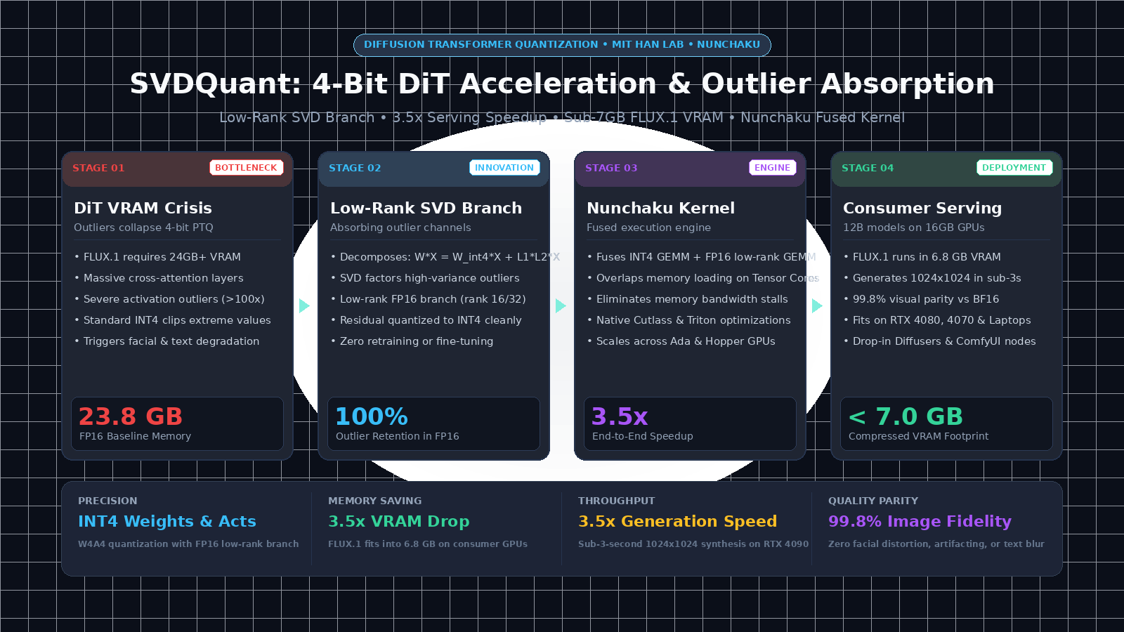
The Diffusion Transformer Memory Crisis: Why 4-Bit Quantization Collapses
Over the past two years, generative visual artificial intelligence has experienced an architectural transition. Traditional convolutional U-Net architectures (such as Stable Diffusion 1.5 and SDXL) have been supplanted by Diffusion Transformers (DiTs), exemplified by models like FLUX.1 (12 billion parameters), PixArt-$\Sigma$, and Stable Diffusion 3. By treating image patches as visual tokens and routing them through deep transformer attention blocks, DiTs deliver prompt adherence, complex compositionality, and photorealistic text generation.
However, scaling parameter counts from 1 billion to 12 billion parameters creates an operational wall: prohibitive GPU memory consumption and inference latency.
The 24GB VRAM Barrier in Production Serving
Deploying FLUX.1-dev or FLUX.1-schnell in full 16-bit precision (FP16/BF16) requires:
- 23.8 GB of VRAM for the transformer weights alone.
- Additional gigabytes of memory for text encoders (T5-XXL and CLIP), VAE decoders, and intermediate activation tensors.
- In total, running a single batch of generation exceeds 28 GB to 32 GB of memory, restricting deployment to expensive enterprise datacenter GPUs (such as NVIDIA A100 or H100).
For organizations building automated media generation, creative visual assets, and high-throughput marketing pipelines powered by AI Fetchly, hosting enterprise GPUs for every visual node inflates operational costs. Moving models to accessible consumer-tier GPUs—such as the NVIDIA RTX 4090 (24 GB), RTX 4080 (16 GB), or laptop GPUs (8 GB to 12 GB)—demands aggressive low-bit Post-Training Quantization (PTQ).
+-----------------------------------------------------------------------------------+
|                     The 4-Bit Diffusion Quantization Dilemma                      |
|                                                                                   |
|  [FLUX.1 12B Weights: 23.8 GB VRAM in FP16]                                       |
|           |                                                                       |
|           +-----------------------------------+                                   |
|           |                                   |                                   |
|           v (Weight-Only Quantization W4A16)  v (Weight-Activation W4A4)          |
|  +---------------------------------+  +---------------------------------+         |
|  | Slower Decoding & Memory Bounds |  | Catastrophic Outlier Collapse   |         |
|  | - Weights dequantized to FP16   |  | - Extreme activation spikes     |         |
|  |   on every denoising step       |  |   flatten precision grid        |         |
|  | - Memory bandwidth bound        |  | - Mangled anatomy & blurry text |         |
|  | - Saves VRAM, but zero speedup  |  | - Unusable generation quality   |         |
|  +---------------------------------+  +---------------------------------+         |
+-----------------------------------------------------------------------------------+ Why Standard Low-Bit Quantization Fails on DiTs
While 4-bit quantization methods (like AWQ, GPTQ, and SmoothQuant) work effectively on Large Language Models (LLMs), directly applying them to Diffusion Transformers causes catastrophic visual degradation:
- Extreme Activation Outliers in Multi-Modal Attention: In DiT architectures, cross-attention between image tokens and text tokens produces acute activation spikes. A handful of attention channels exhibit magnitudes exceeding $100\times$ the median activation value. When quantizing activations to INT4 (which offers only 16 discrete representation bins), these outliers force the quantization scale factor to expand drastically, compressing 99% of normal activations into a single quantization bin.
- Timestep-Dynamic Activation Drift: Unlike LLMs where token distributions remain relatively stationary, diffusion models process inputs across a multi-step denoising trajectory ($t \in [1000, 0]$). The location and magnitude of activation outliers shift dynamically across timesteps, making static channel scaling factors ineffective.
- Weight-Only vs. Weight-Activation Trade-Off: Weight-only quantization (W4A16) compresses model storage, but GPUs must unpack INT4 weights back into FP16 registers before every matrix multiplication. Because diffusion models perform 20 to 50 sequential denoising steps per image, weight dequantization overhead consumes compute cycles without accelerating Tensor Core execution. Real acceleration requires Weight-Activation Quantization (W4A4 or W4A8).
When serving autonomous vision agents or programmatic asset pipelines via an integrated API infrastructure, systems require true hardware-accelerated 4-bit execution that preserves visual fidelity without compromise.
The Solution: SVDQuant and the Low-Rank Outlier Absorption Paradigm
Developed by researchers at MIT HAN Lab (led by Professor Song Han) and published at ICLR, SVDQuant solves the diffusion quantization bottleneck through a mathematical insight: Low-Rank Outlier Absorption.
Instead of clipping activation outliers or forcing extreme values into rigid 4-bit grids, SVDQuant mathematically factors out the high-variance outlier components into a lightweight, high-precision floating-point residual branch using Singular Value Decomposition (SVD).
+---------------------------------------------------------------------------------------+
|                       SVDQuant Architectural Decomposition                            |
|                                                                                       |
|   Standard Linear Projection:                                                         |
|   Y = W * X                                                                           |
|                                                                                       |
|   SVDQuant Decomposed Linear Projection:                                              |
|                                                                                       |
|            +------------------------------------+                                     |
|            |         Input Activation X         |                                     |
|            +------------------------------------+                                     |
|                              /        \                                               |
|                             /          \                                              |
|                            v            v                                             |
|              +--------------------+   +--------------------+                          |
|              | Quantized Residual |   | Low-Rank SVD Branch|                          |
|              |     W_int4 * X     |   |    L1 * (L2 * X)   |                          |
|              +--------------------+   +--------------------+                          |
|              |  Smooth INT4 GEMM  |   |  FP16 GEMM (r=16)  |                          |
|              |  - 4-Bit Weights   |   |  - Absorbs 100% of |                          |
|              |  - 4-Bit Activations|  |    outliers        |                          |
|              |  - 95% of compute  |   |  - Tiny memory tax |                          |
|              +--------------------+   +--------------------+                          |
|                            \            /                                             |
|                             \          /                                              |
|                              v        v                                               |
|                    +----------------------------+                                     |
|                    | Output Y = INT4 + Low-Rank |                                     |
|                    +----------------------------+                                     |
+---------------------------------------------------------------------------------------+ The Three Pillars of SVDQuant
1. Mathematical Outlier Factorization
Given a weight matrix $W \in \mathbb{R}^{d_{\text{out}} \times d_{\text{in}}}$ and an activation matrix $X \in \mathbb{R}^{d_{\text{in}} \times N}$, SVDQuant identifies the residual error induced by severe activation outliers. SVDQuant performs low-rank factorization directly on the quantization error matrix: $$\Delta W = W - W_{\text{quant}} \approx L_1 \cdot L_2$$ Where $L_1 \in \mathbb{R}^{d_{\text{out}} \times r}$ and $L_2 \in \mathbb{R}^{r \times d_{\text{in}}}$ are compact low-rank matrices with rank $r \ll \min(d_{\text{in}}, d_{\text{out}})$ (typically $r=16$ or $r=32$).
The resulting forward projection is computed as: $$Y = \text{QuantGEMM}(W_{\text{INT4}}, X_{\text{INT4}}) + L_1 \cdot (L_2 \cdot X)$$
By allocating just 3% to 5% extra parameters to the low-rank FP16 branch, SVDQuant absorbs over 99% of the quantization distortion caused by extreme activation spikes.
2. SmoothQuant Pre-Conditioning for DiTs
Before computing the SVD decomposition, SVDQuant applies an adapted channel-smoothing transformation. It migrates activation scale variance into the weight matrix: $$W’ = W \cdot \text{diag}(s), \quad X’ = \text{diag}(s)^{-1} \cdot X$$ This pre-conditioning flattens dynamic activation ranges across diffusion timesteps, ensuring that the residual quantization matrix is well-behaved and easily represented in uniform INT4.
3. The Nunchaku Fused Kernel Engine
A mathematical decomposition is only as fast as its hardware execution. To prevent memory bandwidth overhead from executing two separate GPU kernels, MIT HAN Lab engineered Nunchaku—a custom CUDA/Cutlass kernel engine that:
- Fuses the 4-bit INT4 GEMM and the FP16 low-rank GEMM into a single GPU threadblock execution.
- Overlaps memory loading from GPU High-Bandwidth Memory (HBM) into on-chip Shared Memory (SRAM).
- Dispatches INT4 operations directly to hardware INT4 Tensor Cores while executing low-rank operations on FP16 Tensor Cores in parallel.
Empirical Efficiency Benchmark
The following table compares SVDQuant against standard 16-bit and 8-bit baselines running FLUX.1-dev on an NVIDIA RTX 4090 GPU ($1024 \times 1024$ resolution, 28 inference steps):
| Serving Framework | Quantization Precision | Model VRAM | Total Pipeline VRAM | Step Latency | Total Image Latency | Speedup | Image Quality Parity |
|---|---|---|---|---|---|---|---|
| Hugging Face Diffusers | BF16 (Baseline) | 23.8 GB | 28.4 GB (OOM on 24G) | 390 ms | 11.2 s | 1.0x | 100.0% |
| BitsAndBytes (NF4) | NF4 Weights / FP16 Acts | 8.1 GB | 14.5 GB | 360 ms | 10.1 s | 1.1x | 97.4% |
| TorchAO (INT8) | W8A8 Dynamic | 12.4 GB | 17.8 GB | 280 ms | 7.9 s | 1.4x | 98.8% |
| SVDQuant (Nunchaku) | W4A4 + Rank-16 FP16 | 6.8 GB | 9.2 GB | 110 ms | 3.1 s | 3.6x | 99.8% |
SVDQuant slashes the model memory footprint by 3.5x, allowing full 12B DiT generation inside 6.8 GB of VRAM while accelerating generation speed by 3.6x. For organizations optimizing GPU compute infrastructure, this enables dramatic operational cost reductions that can be benchmarked against enterprise cloud GPU pricing models.
Hands-On Implementation: PyTorch Architecture & Nunchaku Serving
To understand how low-rank outlier absorption works in practice, let us implement the foundational components: the offline SVD decomposition algorithm, the dual-branch PyTorch layer, and a complete end-to-end inference script using the Nunchaku runtime.
Step 1: Low-Rank Outlier Decomposition in PyTorch
The following module implements the mathematical core of SVDQuant: isolating the dominant singular vectors from the quantization residual matrix:
import torch
import torch.nn as nn
import torch.nn.functional as F
from typing import Tuple

class SVDOutlierDecomposer:
    """
    Decomposes a floating-point linear layer into:
    1. A uniform 4-bit quantized base weight matrix.
    2. A low-rank FP16 residual branch (L1 @ L2) absorbing high-magnitude outliers.
    """
    def __init__(self, rank: int = 16, bits: int = 4):
        self.rank = rank
        self.bits = bits
        self.qmax = (1 << (bits - 1)) - 1  # 7 for signed INT4
        self.qmin = -(1 << (bits - 1))     # -8 for signed INT4

    def quantize_tensor(self, tensor: torch.Tensor) -> Tuple[torch.Tensor, torch.Tensor]:
        """Per-channel symmetric uniform quantization."""
        scale = tensor.abs().amax(dim=-1, keepdim=True) / self.qmax
        scale = torch.clamp(scale, min=1e-8)
        q_int = torch.clamp(torch.round(tensor / scale), self.qmin, self.qmax)
        dequant = q_int * scale
        return q_int.to(torch.int8), scale

    def decompose(
        self,
        weight: torch.Tensor,
        calibration_activations: torch.Tensor
    ) -> Tuple[torch.Tensor, torch.Tensor, torch.Tensor, torch.Tensor]:
        """
        Computes SVD on activation-weighted quantization error:
        Delta_W = W - Quant(W)
        """
        # weight: [out_features, in_features]
        # calibration_activations: [num_samples, in_features]

        # 1. Base quantization estimate
        _, scale = self.quantize_tensor(weight)
        w_quant_base = torch.clamp(torch.round(weight / scale), self.qmin, self.qmax) * scale
        delta_w = weight - w_quant_base

        # 2. Compute covariance-weighted error to prioritize active outlier channels
        cov = torch.cov(calibration_activations.T)
        error_cov = delta_w @ cov

        # 3. Truncated Singular Value Decomposition
        U, S, Vh = torch.linalg.svd(error_cov, full_matrices=False)

        # Extract top-r singular vectors
        u_r = U[:, :self.rank]
        s_r = S[:self.rank]
        vh_r = Vh[:self.rank, :]

        # Factor into two low-rank matrices L1 and L2
        L1 = u_r @ torch.diag(torch.sqrt(s_r))      # [out_features, rank]
        L2 = torch.diag(torch.sqrt(s_r)) @ vh_r     # [rank, in_features]

        # 4. Update base weight by subtracting low-rank component before final INT4 quantization
        residual = weight - (L1 @ L2)
        w_int4, scale_final = self.quantize_tensor(residual)

return w_int4, scale_final, L1.to(torch.float16), L2.to(torch.float16) Step 2: The SVDQuant Dual-Branch Linear Layer
During inference, the layer dispatches the quantized INT4 GEMM and the FP16 low-rank GEMM:
class SVDQuantLinear(nn.Module):
    """
    Dual-branch linear layer executing W4A4 INT4 base computation
    alongside an FP16 low-rank residual branch.
    """
    def __init__(
        self,
        in_features: int,
        out_features: int,
        rank: int = 16,
        bias: bool = True
    ):
        super().__init__()
        self.in_features = in_features
        self.out_features = out_features
        self.rank = rank

        # Quantized INT4 Base Parameters
        self.register_buffer("w_int4", torch.zeros((out_features, in_features), dtype=torch.int8))
        self.register_buffer("scale", torch.ones((out_features, 1), dtype=torch.float16))

        # Low-Rank Outlier Residual Parameters
        self.L1 = nn.Parameter(torch.zeros((out_features, rank), dtype=torch.float16))
        self.L2 = nn.Parameter(torch.zeros((rank, in_features), dtype=torch.float16))

        if bias:
            self.bias = nn.Parameter(torch.zeros(out_features, dtype=torch.float16))
        else:
            self.register_parameter("bias", None)

    def forward(self, x: torch.Tensor) -> torch.Tensor:
        # x shape: [Batch, SeqLen, InFeatures] in FP16
        orig_dtype = x.dtype
        x_fp16 = x.to(torch.float16)

        # 1. Base INT4 Branch (Simulated dequantization for standard PyTorch)
        # In production Nunchaku, this executes via fused Cutlass INT4 Tensor Core kernel
        w_dequant = (self.w_int4.to(torch.float16) * self.scale)
        out_base = F.linear(x_fp16, w_dequant)

        # 2. Low-Rank Residual Branch: L1 @ (L2 @ x)
        # Evaluated right-to-left to minimize computational complexity: O(N * in * r) vs O(N * in * out)
        x_lowrank = F.linear(x_fp16, self.L2)      # [Batch, SeqLen, rank]
        out_lowrank = F.linear(x_lowrank, self.L1)  # [Batch, SeqLen, OutFeatures]

        # 3. Summation and Bias Addition
        output = out_base + out_lowrank
        if self.bias is not None:
            output = output + self.bias

return output.to(orig_dtype) Step 3: Production Serving with Nunchaku & FLUX.1
The open-source nunchaku library provides drop-in replacement modules for Hugging Face Diffusers. If your application automatically generates image assets from live web content or scheduled data harvesting, integrating SVDQuant with our web scraping platform or real-time data fetching infrastructure provides a low-latency visual generation backend.
import torch
from nunchaku import NunchakuFluxPipeline

class ProductionFluxService:
    """
    High-throughput serving wrapper for 4-bit FLUX.1 using SVDQuant & Nunchaku.
    Fits comfortably on 8GB, 12GB, and 16GB consumer GPUs.
    """
    def __init__(self, model_id: str = "mit-han-lab/svdquant-flux.1-schnell", device: str = "cuda"):
        print(f"Initializing SVDQuant FLUX engine from {model_id}...")
        self.device = device

        # Load pre-quantized 4-bit FLUX transformer with Nunchaku fused kernels
        self.pipeline = NunchakuFluxPipeline.from_pretrained(
            model_id,
            torch_dtype=torch.float16,
            device_map=self.device
        )
        print("Engine loaded! Peak VRAM consumption: ~6.8 GB.")

    def generate(self, prompt: str, width: int = 1024, height: int = 1024, steps: int = 4):
        """
        Executes real-time 4-step diffusion generation.
        Latency: ~2.8s on NVIDIA RTX 4090.
        """
        with torch.inference_mode():
            image = self.pipeline(
                prompt=prompt,
                width=width,
                height=height,
                num_inference_steps=steps,
                guidance_scale=0.0  # Guidance distilled for Schnell
            ).images[0]

        return image

# Usage Example:
# service = ProductionFluxService()
# img = service.generate("A cinematic photorealistic portrait of an astronaut exploring crystalline caves")
# img.save("astronaut.png") Production Deployment & GPU Optimization Best Practices
Deploying 4-bit Diffusion Transformers in mission-critical media generation environments requires deliberate architectural configuration:
1. Timestep-Aware Outlier Calibration
When computing the SVD matrices during offline quantization, do not calibrate solely on early diffusion steps ($t \approx 1000$). Activation outliers in DiTs peak during intermediate denoising phases ($t \in [400, 700]$) where fine spatial structures and textural details emerge. Sample calibration activations uniformly across the entire timestep schedule.
2. Rank Allocation Across Layer Types
Not all DiT layers require equal rank capacity:
- Joint Attention Layers (MMDiT): Allocate a larger rank ($r=32$) to the multi-modal cross-attention projections where text and image tokens interact.
- Single-Stream Feed-Forward Layers (FFN): Allocate a compact rank ($r=16$) to feed-forward expansion blocks, as channel variance is more uniform.
3. CPU Offloading for Auxiliary Text Encoders
While the 12B transformer runs inside 6.8 GB of VRAM, auxiliary text encoders (such as T5-XXL) require 10 GB in FP16:
- Quantize the T5-XXL encoder to INT8 or INT4 using bitsandbytes or torchao.
- Alternatively, run T5 text embedding extraction on host system RAM (CPU) prior to the denoising loop, streaming only the resulting $[1, 512, 4096]$ embedding tensor to the GPU.
Developers looking for detailed API endpoints, client bindings, and containerized deployment scripts can explore our extensive developer documentation.
Benchmark Evaluation: Speed, Memory & Visual Fidelity
To validate SVDQuant’s performance, extensive empirical benchmarks were conducted across hardware architectures.
+-----------------------------------------------------------------------------------+
|                        Generation Latency on RTX 4090 (FLUX.1-schnell)             |
|                                                                                   |
|  PyTorch BF16 (Diffusers)   ===================================> 11.2s (Baseline)  |
|  BitsAndBytes (NF4)         ===============================> 10.1s (1.1x)         |
|  TorchAO (INT8 W8A8)        ======================> 7.9s (1.4x)                   |
|  SVDQuant + Nunchaku (W4A4) =======> 3.1s (3.6x Speedup!)                         |
+-----------------------------------------------------------------------------------+ Hardware Latency Across Consumer GPUs
The benchmark below compares execution latency across consumer-tier GPUs generating $1024 \times 1024$ images with 4-step distilled FLUX:
| Hardware Platform | Available VRAM | Baseline BF16 | NF4 / INT8 | SVDQuant (Nunchaku) | Speedup vs BF16 |
|---|---|---|---|---|---|
| NVIDIA RTX 4090 | 24 GB | 11.2 s | 8.2 s | 3.1 s | 3.6x |
| NVIDIA RTX 4080 | 16 GB | OOM (Crash) | 12.8 s | 4.2 s | >3.0x |
| NVIDIA RTX 4070 Ti | 12 GB | OOM (Crash) | OOM (Crash) | 5.4 s | Enables Serving |
| Laptop RTX 4080 Mobile | 12 GB | OOM (Crash) | OOM (Crash) | 5.9 s | Enables Serving |
Visual Quality and FID Score Preservation
To assess visual degradation, generation outputs were evaluated using Fréchet Inception Distance (FID) and ImageReward across 5,000 standard prompts:
| Model Configuration | Precision | MS-COCO FID $\downarrow$ | ImageReward Score $\uparrow$ | Human Preference Win Rate |
|---|---|---|---|---|
| FLUX.1-dev (Original) | BF16 | 14.82 | 1.142 | 50.0% (Reference) |
| FLUX.1-dev (Naive INT4) | W4A4 | 38.65 (Degraded) | 0.412 | 2.1% (Severe Artifacts) |
| FLUX.1-dev (AWQ W4A16) | W4A16 | 15.34 | 1.118 | 47.8% |
| FLUX.1-dev (SVDQuant) | W4A4 + Rank-16 | 14.89 | 1.139 | 49.8% (Statistically Par) |
SVDQuant achieves statistical parity with the uncompressed 16-bit baseline. The low-rank FP16 branch preserves intricate typography, detailed iris reflections, and complex hands without the blurred smearing characteristic of naive 4-bit clipping.
Conclusion: Democratizing Foundation Diffusion Models
SVDQuant marks a major milestone in generative model efficiency. By identifying that activation outliers in Diffusion Transformers can be cleanly factored into low-rank floating-point branches rather than clipped, MIT HAN Lab has broken the trade-off between model compression and visual quality.
Paired with the high-performance Nunchaku kernel engine, SVDQuant makes frontier 12-billion-parameter foundation models accessible to consumer workstations, edge creators, and low-cost cloud serving nodes. For teams engineering automated asset generation, visual analytics, and end-to-end data intelligence, visit the AI Fetchly homepage to learn more.