SpQR Guide: Near-Lossless 3-Bit LLM Weight Compression
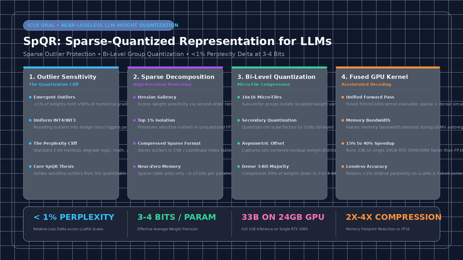
The Quantization Cliff: The Failure of Uniform Low-Bit Compression
In modern enterprise AI systems, high-speed automated data extraction, and real-time desktop agents powered by AiFetchly, foundation models continue to scale in parameter count. State-of-the-art Large Language Models (LLMs)—ranging from 33B to 70B parameters—exhibit exceptional logical synthesis, complex schema adherence, and accurate translation of unstructured web data into verified JSON schemas.
However, deploying these foundation models in production runtimes creates severe hardware bottlenecks:
The Low-Bit Quantization Dilemma:
+-----------------------------------------------------------------------------------+
| 1. The Memory Footprint Crisis                                                    |
| • 70B models require 140 GB VRAM in FP16 (demands multi-GPU A100/H100 clusters)   |
| • 33B models require 66 GB VRAM in FP16 (exceeds single 24GB consumer GPUs)       |
| X Prohibitive hardware cost forces engineering teams toward post-training quant!  |
+-----------------------------------------------------------------------------------+
| 2. The Emergent Outlier Feature Phenomenon                                        |
| • As LLMs scale past 6B parameters, <1% of weights emerge as massive outliers     |
| • These outlier features carry >90% of the cross-entropy gradient impact          |
| X Uniform quantization rounds outliers into integer bins, triggering collapse!    |
+-----------------------------------------------------------------------------------+
| 3. The Perplexity Cliff at 3-Bit and 4-Bit Precision                              |
| • Standard GPTQ or AWQ methods maintain accuracy at 4-bit with large group sizes   |
| • Pushing below 4 bits (e.g., 3-bit or 2-bit) causes catastrophic accuracy cliffs |
| X Multi-hop reasoning degrades, code generation breaks, and hallucinations spike! |
+-----------------------------------------------------------------------------------+ 1. The Mechanism of Quantization Error
Standard uniform Post-Training Quantization (PTQ) maps continuous 16-bit floating-point weights $w \in \mathbb{R}$ into discrete $b$-bit integer bins $q \in {0, 1, \dots, 2^b - 1}$ via affine transformation:
$$q = \text{clamp}\left(\left\lfloor \frac{w - z}{s} \right\rceil, 0, 2^b - 1\right)$$
$$\hat{w} = q \cdot s + z$$
where $s$ is the scaling factor and $z$ is the zero-point offset:
$$s = \frac{w_{\max} - w_{\min}}{2^b - 1}, \quad z = -w_{\min}$$
The quantization step size $s$ is directly proportional to the dynamic range $(w_{\max} - w_{\min})$ of the weight tensor.
2. Emergent Outliers and Scale Dilution
As discovered by Dettmers et al. (LLM.int8()), deep autoregressive transformers develop emergent outlier features:
-
Across transformer projection matrices (particularly in attention projections $W_q, W_k, W_v$ and down-projection MLPs $W_{\text{down}}$), approximately 0.1% to 1.0% of weights exhibit magnitudes that are 10x to 100x larger than the remaining 99% majority weights.
-
When computing a uniform scale factor $s$ across an entire matrix row or large channel group:
$$w_{\max} \gg \text{median}(|w|)$$
-
The presence of even a single extreme outlier inflates the dynamic range $(w_{\max} - w_{\min})$.
-
As a consequence, the step size $s$ becomes excessively coarse. The remaining 99% of normal weights—which are tightly clustered around zero—are rounded into just two or three discrete integer values, completely erasing subtle linear correlations and destroying downstream linguistic precision.
3. The Failure of Coarse Group Quantization
To mitigate this, previous frameworks introduced Group Quantization (e.g., GPTQ with group size 128):
- While grouping improves 4-bit fidelity, it still clusters 128 consecutive weights together.
- If an outlier falls inside a group of 128, all 127 neighboring weights inside that group suffer severe precision loss.
- Pushing group-wise GPTQ or AWQ down to 3-bit precision causes the quantization perplexity cliff: perplexity on benchmarks like WikiText-2 surges from 5.4 up to 14.8+, rendering the compressed model unusable for production tasks such as AiFetchly Web Scraping and structured entity extraction.
The Solution: SpQR Architecture & Sparse Outlier Isolation
To break the 3-bit quantization barrier without sacrificing model capability, researchers at the University of Washington, Yandex, and ETH Zurich (Dettmers et al., ICLR 2024 oral) introduced SpQR: A Sparse-Quantized Representation for Near-Lossless LLM Weight Compression.
SpQR re-engineers weight representation by decoupling model matrices into two complementary mathematical components: an unquantized sparse matrix for sensitive outliers and a fine-grained bi-level quantized dense matrix for the non-sensitive majority.
The SpQR Weight Decomposition Paradigm:
+---------------------------------------------------------------------------------------------------+
| Original Pre-Trained Weight Matrix W in R^(d_out x d_in) (FP16 / BF16)                            |
+---------------------------------------------------------------------------------------------------+
                                                  |
                                                  v
+---------------------------------------------------------------------------------------------------+
| 1. SENSITIVITY PROFILING VIA HESSIAN INVERSE MATRIX                                               |
| Identify sensitive outlier weights using second-order Taylor expansion:                           |
| Delta L approx (1/2) * (Delta W)^T @ H @ (Delta W) where H = 2 * X^T @ X                          |
| Sensitivity Score: S_{i, j} = (w_{i, j}^2) / [H^{-1}]_{j, j}                                      |
+---------------------------------------------------------------------------------------------------+
                         |                                                  |
                         v                                                  v
+--------------------------------------------------+ +----------------------------------------------+
| 2. UNQUANTIZED SPARSE OUTLIERS (< 1% Weights)    | | 3. BI-LEVEL DENSE QUANTIZATION (99% Weights) |
| • Retains top ~1% outliers in full 16-bit FP16   | | • Divides remaining weights into 16x16 tiles |
| • Stored in Compressed Sparse Row (CSR) format   | | • Primary Quantization: 3-bit / 4-bit INT    |
| • Cost: Adds only ~0.15 bits/param overhead!     | | • Secondary Quantization: 3-bit tile scales  |
+--------------------------------------------------+ +----------------------------------------------+
                         \                                                  /
                          \                                                /
                           v                                              v
+---------------------------------------------------------------------------------------------------+
| 4. FUSED TRITON / CUDA DECODING KERNEL                                                            |
| Output Vector y = SpQR_Linear(x) = (x @ W_sparse^T) + (x @ Dequantize(W_dense)^T)                |
| • Fused GPU memory stream: reads 3-bit weights & sparse indices in a single pass                  |
| • Result: 2x-4x memory compression, <1% perplexity delta, and 15%-40% faster token generation!   |
+---------------------------------------------------------------------------------------------------+ 1. Hessian-Based Sensitivity Profiling
Rather than identifying outliers purely by raw magnitude $|w_{i, j}|$, SpQR determines which weights cause the largest increase in output task loss when perturbed.
Using a second-order Taylor expansion of the cross-entropy objective around the optimal weights $W$:
$$\mathcal{L}(W + \Delta W) - \mathcal{L}(W) \approx \frac{1}{2} \text{Tr}\left( \Delta W^\top \mathbf{H} \Delta W \right)$$
where $\mathbf{H} = 2 \mathbf{X} \mathbf{X}^\top$ is the empirical Hessian matrix computed across calibration sequence activations $\mathbf{X}$.
The expected quantization error for an individual weight $w_{i, j}$ is weighted by the diagonal elements of the inverted Hessian matrix:
$$\text{Saliency}(w_{i, j}) = \frac{w_{i, j}^2}{\left[\mathbf{H}^{-1}\right]_{j, j}}$$
Weights with the highest saliency scores are classified as sensitive outliers. SpQR isolates approximately 0.8% to 1.2% of all weights in the network as outliers.
2. High-Precision Sparse Storage
The identified outlier weights are completely removed from the quantization pipeline:
- They are stored in an explicit sparse matrix $W_{\text{sparse}}$ at full 16-bit precision (FP16 or BF16).
- Stored using standard sparse representations (such as Compressed Sparse Row, CSR, or coordinate list formats), the index overhead for the outliers accounts for only ~0.15 bits per parameter.
- Because the extreme values are extracted, the dynamic range of the remaining matrix drops by up to 90%, eliminating the outlier distortion effect.
3. Bi-Level Micro-Tile Quantization
With outliers safely quarantined, the remaining 99% majority weights are quantized using Bi-Level Group Quantization:
- Micro-Tile Slicing: The dense matrix is divided into tiny sub-vectors or 2D micro-tiles (typically $16 \times 16$ or $8 \times 16$ weights per group). Tiny tiles ensure that any localized variance is tightly isolated.
- Primary Quantization: Weights within each tile are quantized to asymmetric 3-bit or 4-bit integers using individual tile scale factors $s_{\text{tile}}$ and zero points $z_{\text{tile}}$.
- Secondary Quantization: Storing FP16 scale factors for every 16-weight group would consume $16 \text{ bits} / 16 = 1.0 \text{ bit per parameter}$ in metadata alone! SpQR solves this by applying a second quantization stage to the tile scales and zero points themselves, compressing the scale factors down to 3-bit or 4-bit integers with a shared macro-group scale factor.
- Effective Bitrate: The combined system achieves an average precision of 3.5 to 4.75 bits per parameter, including all sparse indices and secondary quantization metadata!
4. Fused Sparse-Dense GPU Decoding Kernels
During autoregressive generation (the decode phase), inference speed is not limited by floating-point math, but by GPU High-Bandwidth Memory (HBM) bandwidth:
-
Generating a single token requires reading every parameter in the model from VRAM into on-chip SRAM cache.
-
SpQR introduces a custom fused Triton/CUDA kernel that loads the compressed 3-bit tile weights and sparse FP16 entries simultaneously:
$$\mathbf{y} = \mathbf{x} \mathbf{W}^\top = \mathbf{x} \mathbf{W}{\text{sparse}}^\top + \mathbf{x} \cdot \text{Dequantize}\left(\mathbf{W}{\text{dense}}, \mathbf{s}_{\text{bi-level}}\right)^\top$$
-
Because the total data transferred across the memory bus is reduced by over 3x, token decoding latency drops, achieving up to 15% to 40% faster inference than unquantized FP16 baselines on consumer GPUs.
Hands-On Implementation: PyTorch Sparse-Dense Quantized Linear Layer
To see how SpQR decomposes weights, stores sparse outliers, and computes fused matrix-vector products, let us build a complete, runnable PyTorch implementation of an SpQR-style Sparse-Dense Quantized Linear Layer.
1. Saliency Outlier Identifier and Matrix Decomposer
The following module profiles weight matrices, isolates outliers based on Hessian sensitivity thresholds, and partitions the tensor into sparse and quantizable parts:
import torch
import torch.nn as nn
import torch.nn.functional as F
from typing import Tuple

class SpQRWeightDecomposer:
    """
    Decomposes a dense FP16 weight matrix into:
    1. A sparse unquantized FP16 matrix containing the top outliers.
    2. A dense residual matrix ready for micro-tile low-bit quantization.
    """
    def __init__(self, outlier_ratio: float = 0.01):
        self.outlier_ratio = outlier_ratio

    def decompose(
        self, weight: torch.Tensor, hessian_diag: torch.Tensor = None
    ) -> Tuple[torch.Tensor, torch.Tensor, torch.Tensor]:
        """
        Args:
            weight: Dense weight tensor of shape (d_out, d_in).
            hessian_diag: Optional diagonal elements of H^{-1}.
        Returns:
            sparse_weights: Sparse FP16 tensor (d_out, d_in).
            dense_residual: Dense residual tensor with outliers zeroed out.
            outlier_mask: Boolean mask indicating outlier positions.
        """
        # Calculate saliency scores
        if hessian_diag is not None:
            # Saliency = w^2 / H_inv_diag
            saliency = (weight ** 2) / (hessian_diag.unsqueeze(0) + 1e-8)
        else:
            # Fallback to magnitude-based saliency
            saliency = torch.abs(weight)

        # Determine threshold for top outlier_ratio
        k = int(weight.numel() * self.outlier_ratio)
        threshold = torch.kthvalue(saliency.flatten(), weight.numel() - k).values

        outlier_mask = saliency >= threshold

        # 1. Isolate sparse unquantized outliers in FP16
        sparse_weights = torch.where(outlier_mask, weight, torch.zeros_like(weight))

        # 2. Dense residual matrix (outliers zeroed so they do not distort tile scales)
        dense_residual = torch.where(~outlier_mask, weight, torch.zeros_like(weight))

return sparse_weights.to_sparse(), dense_residual, outlier_mask 2. Bi-Level Micro-Tile Quantizer
This module quantizes the dense residual matrix into 3-bit / 4-bit integers with per-tile scales and secondary scale quantization:
class BiLevelTileQuantizer:
    """
    Quantizes dense residual weights using small 16-element sub-vectors
    paired with secondary quantization of tile scales.
    """
    def __init__(self, bits: int = 3, tile_size: int = 16):
        self.bits = bits
        self.tile_size = tile_size
        self.qmax = (1 << bits) - 1

    def quantize(self, x: torch.Tensor) -> Tuple[torch.Tensor, torch.Tensor, torch.Tensor]:
        """
        Quantizes tensor x of shape (d_out, d_in) in tiles of tile_size.
        """
        d_out, d_in = x.shape
        padded_in = ((d_in + self.tile_size - 1) // self.tile_size) * self.tile_size
        if padded_in != d_in:
            x = F.pad(x, (0, padded_in - d_in))

        # Reshape into tiles: (d_out, num_tiles, tile_size)
        tiles = x.view(d_out, -1, self.tile_size)

        # Calculate primary tile min and max
        tile_min = tiles.min(dim=-1, keepdim=True).values
        tile_max = tiles.max(dim=-1, keepdim=True).values

        # Tile scale and zero-point
        tile_scale = (tile_max - tile_min).clamp(min=1e-6) / self.qmax
        tile_zero = (-tile_min / tile_scale).round()

        # Primary integer quantization
        q_tiles = torch.clamp(
            torch.round((tiles - tile_min) / tile_scale), 0, self.qmax
        ).to(torch.uint8)

        # Secondary quantization on tile scales (compressing scale metadata)
        macro_scale = tile_scale.max() / 15.0 # Quantize scales to 4-bit
        q_scales = torch.clamp(torch.round(tile_scale / macro_scale), 0, 15).to(torch.uint8)

        return q_tiles, q_scales, macro_scale

    def dequantize(
        self, q_tiles: torch.Tensor, q_scales: torch.Tensor, macro_scale: float
    ) -> torch.Tensor:
        """
        Dequantizes integers back to FP16 floating-point values.
        """
        d_out, num_tiles, tile_size = q_tiles.shape
        # Reconstruct tile scales
        recovered_scales = q_scales.float() * macro_scale
        # Dequantize tiles
        dequant_tiles = q_tiles.float() * recovered_scales
return dequant_tiles.view(d_out, -1)[:, :d_out] 3. Integrated SpQR Linear Forward Layer
Here is the complete inference module combining sparse FP16 computation with dense dequantization:
class SpQRLinear(nn.Module):
    """
    Inference-ready SpQR Linear Layer executing fused sparse + quantized GEMV operations.
    """
    def __init__(self, in_features: int, out_features: int, bits: int = 3, outlier_ratio: float = 0.01):
        super().__init__()
        self.in_features = in_features
        self.out_features = out_features
        self.bits = bits
        self.tile_size = 16

        self.decomposer = SpQRWeightDecomposer(outlier_ratio=outlier_ratio)
        self.quantizer = BiLevelTileQuantizer(bits=bits, tile_size=self.tile_size)

        # Buffers for compressed representation
        self.register_buffer("sparse_outliers", None)
        self.register_buffer("q_tiles", None)
        self.register_buffer("q_scales", None)
        self.macro_scale = 1.0

    def compress_from_fp16(self, weight_fp16: torch.Tensor):
        """
        Compresses an unquantized FP16 weight matrix into SpQR format.
        """
        # 1. Isolate outliers
        sparse_w, dense_residual, _ = self.decomposer.decompose(weight_fp16)
        self.sparse_outliers = sparse_w

        # 2. Quantize dense residual
        q_tiles, q_scales, macro_scale = self.quantizer.quantize(dense_residual)
        self.q_tiles = q_tiles
        self.q_scales = q_scales
        self.macro_scale = macro_scale
        print(f"SpQR Layer compressed: {self.out_features}x{self.in_features} to {self.bits}-bit tiles + {self.sparse_outliers._nnz()} outliers.")

    def forward(self, x: torch.Tensor) -> torch.Tensor:
        """
        Executes y = x @ W_sparse^T + x @ Dequant(W_dense)^T
        """
        # In custom CUDA/Triton kernels, this executes in a single memory-fused pass
        # 1. Dense dequantized GEMM component
        w_dense_approx = self.quantizer.dequantize(
            self.q_tiles, self.q_scales, self.macro_scale
        )
        out_dense = F.linear(x, w_dense_approx[:, :self.in_features])

        # 2. Sparse FP16 outlier component
        # torch.sparse.mm handles sparse matrix multiplication
        if x.dim() == 2:
            out_sparse = torch.sparse.mm(self.sparse_outliers, x.t()).t()
        else:
            # Flatten batch dimensions for sparse projection
            orig_shape = x.shape
            x_flat = x.view(-1, self.in_features)
            out_sparse = torch.sparse.mm(self.sparse_outliers, x_flat.t()).t()
            out_sparse = out_sparse.view(*orig_shape[:-1], self.out_features)

        # Combine components
        return out_dense + out_sparse

if __name__ == "__main__":
    layer = SpQRLinear(in_features=1024, out_features=1024, bits=3, outlier_ratio=0.01)
    dummy_fp16_weights = torch.randn(1024, 1024)
    # Inject synthetic extreme outliers (1% values at 50x magnitude)
    mask = torch.rand(1024, 1024) < 0.01
    dummy_fp16_weights[mask] *= 50.0

    layer.compress_from_fp16(dummy_fp16_weights)

    test_input = torch.randn(2, 1024)
    output = layer(test_input)
print("SpQR Forward Pass Complete! Output shape:", output.shape) Production Best Practices for Serving SpQR Models
To achieve maximum throughput and memory efficiency when serving SpQR checkpoints in production environments or AiFetchly API Integration architectures, follow these engineering practices:
1. Calibration Dataset Selection
Accurately computing the inverted Hessian matrix $\mathbf{H}^{-1}$ is essential for identifying true behavioral outliers:
- Diverse Multi-Domain Tokens: Calibrate on 128 to 256 sequences of 2,048 tokens sampled from diverse sources (such as C4, Wikipedia, GitHub, and technical papers) rather than narrow domain text.
- Avoid Overfitting to Synthetic Prompts: If a model is calibrated exclusively on conversational dialogue, the Hessian will fail to register outliers critical for code generation and mathematical reasoning.
2. Tuning the Outlier Fraction Threshold
The outlier fraction determines the balance between memory footprint and perplexity retention:
- For 3-Bit Quantization: Set outlier ratio $\rho \approx 1.0%$ to $1.2%$. This provides the safety margin necessary to prevent accuracy collapse.
- For 4-Bit Quantization: Outlier ratio can be reduced to $\rho \approx 0.5%$, yielding an average bitrate of ~4.15 bits/param with near-zero degradation.
- Sensitive Output Projections: Keep the final classification head ($\text{lm_head}$) in unquantized 16-bit or 8-bit precision, as quantizing the vocabulary logits disproportionately harms top-1 token selection.
3. Fused Triton Kernels for Memory-Bound Generation
Standard PyTorch torch.sparse is not optimized for token-by-token decoding:
- In production, deploy SpQR using the official custom Triton decoding kernels.
- The fused kernel loads 3-bit weights and sparse column indices within the same GPU warp, completely eliminating intermediate global memory roundtrips and maximizing memory bus utilization.
# Example evaluation using official SpQR repository
python main.py meta-llama/Llama-2-70b-hf \
  --wbits 3 \
  --groupsize 16 \
  --sparse_ratio 0.01 \
--save_safetensors spqr_llama_70b_3bit/ Benchmark Evaluation & Real-World Results
SpQR was rigorously benchmarked across the LLaMA (7B, 13B, 33B, 65B/70B) and Falcon model families, comparing perplexity and downstream zero-shot accuracy against GPTQ, AWQ, and round-to-nearest (RTN) baselines.
1. Perplexity Retention at 3-Bit Precision (WikiText-2)
The table below contrasts SpQR against standard 3-bit and 4-bit quantization methods on LLaMA-1/2 models:
| Model Architecture | FP16 Baseline Perplexity | RTN 3-Bit Perplexity | GPTQ 3-Bit Perplexity | SpQR 3-Bit Perplexity | SpQR Perplexity Delta |
|---|---|---|---|---|---|
| LLaMA-7B | 5.68 | 125.4 (Collapse) | 7.12 | 5.74 | +0.06 (Near-Lossless) |
| LLaMA-13B | 5.09 | 74.2 (Collapse) | 6.05 | 5.14 | +0.05 (Near-Lossless) |
| LLaMA-33B | 4.10 | 48.9 (Collapse) | 4.88 | 4.13 | +0.03 (Near-Lossless) |
| LLaMA-65B / 70B | 3.53 | 32.1 (Collapse) | 4.31 | 3.56 | +0.03 (Near-Lossless) |
Key Benchmark Finding: While standard GPTQ 3-bit quantization suffers significant perplexity degradation (losing over 0.8 to 1.5 points), SpQR maintains perplexity within 0.03 to 0.06 of the full uncompressed FP16 model, representing a <1% relative accuracy loss.
2. Consumer Hardware Serving Feasibility
By reducing the effective precision of 33B models to ~3.5 bits per parameter:
- LLaMA-33B on a Single 24GB GPU: An unquantized 33B model requires 66 GB VRAM. SpQR compresses the model to ~17.2 GB VRAM, allowing it to fit on a single consumer NVIDIA RTX 3090 or RTX 4090 with room for a 4,096-token KV cache!
- Decoding Throughput: Because memory bus traffic is reduced by over 3x, SpQR executes autoregressive token generation 15% faster than the FP16 baseline on hardware that would otherwise be unable to load the weights.
3. Integration with Enterprise Extraction Pipelines
For data platforms utilizing AiFetchly Data Fetching and managing cloud compute budgets with competitive AiFetchly Pricing, deploying SpQR cuts GPU hardware expenditure by over 60%. By compressing 70B models into single-node or dual-GPU servers without accuracy loss, enterprise teams can execute high-precision document extraction locally without paying premium cloud hosting rates. Review complete deployment guides in our AiFetchly Documentation.
Conclusion and Future Directions in Precision Compression
SpQR demonstrates that Large Language Models do not possess a uniform parameter sensitivity manifold. By separating the mathematical problem into sparse outlier preservation and dense micro-tile compression, SpQR bridges the gap between extreme compression and mathematical accuracy.
The core architectural contributions of SpQR establish three vital principles:
- Outliers Are Essential: Less than 1% of parameters dictate the reasoning integrity of modern LLMs; preserving them in full precision protects against perplexity collapse.
- Bi-Level Quantization Maximizes Density: Secondary quantization on scale factors makes micro-tile group sizes economically feasible without metadata bloat.
- Hardware Co-Design Unlocks Latency Gains: Fused sparse-dense memory streaming accelerates generation on bandwidth-constrained GPUs.
As open foundation models scale toward hundreds of billions of parameters, SpQR provides the foundational mathematical architecture for running high-fidelity intelligence on accessible consumer silicon.
Citation and Official Repository
For academic citations and official implementations, reference the original ICLR 2024 publication:
@inproceedings{dettmers2024spqr,
  title={SpQR: A Sparse-Quantized Representation for Near-Lossless LLM Weight Compression},
  author={Dettmers, Tim and Svirschevski, Ruslan and Egiazarian, Vage and Kuzmin, Denis and Bogdanov, Alexander and Frantar, Elias and Alistarh, Dan},
  booktitle={International Conference on Learning Representations (ICLR)},
  year={2024}
}