Sophia Guide: Second-Order Stochastic Optimizer for LLMs

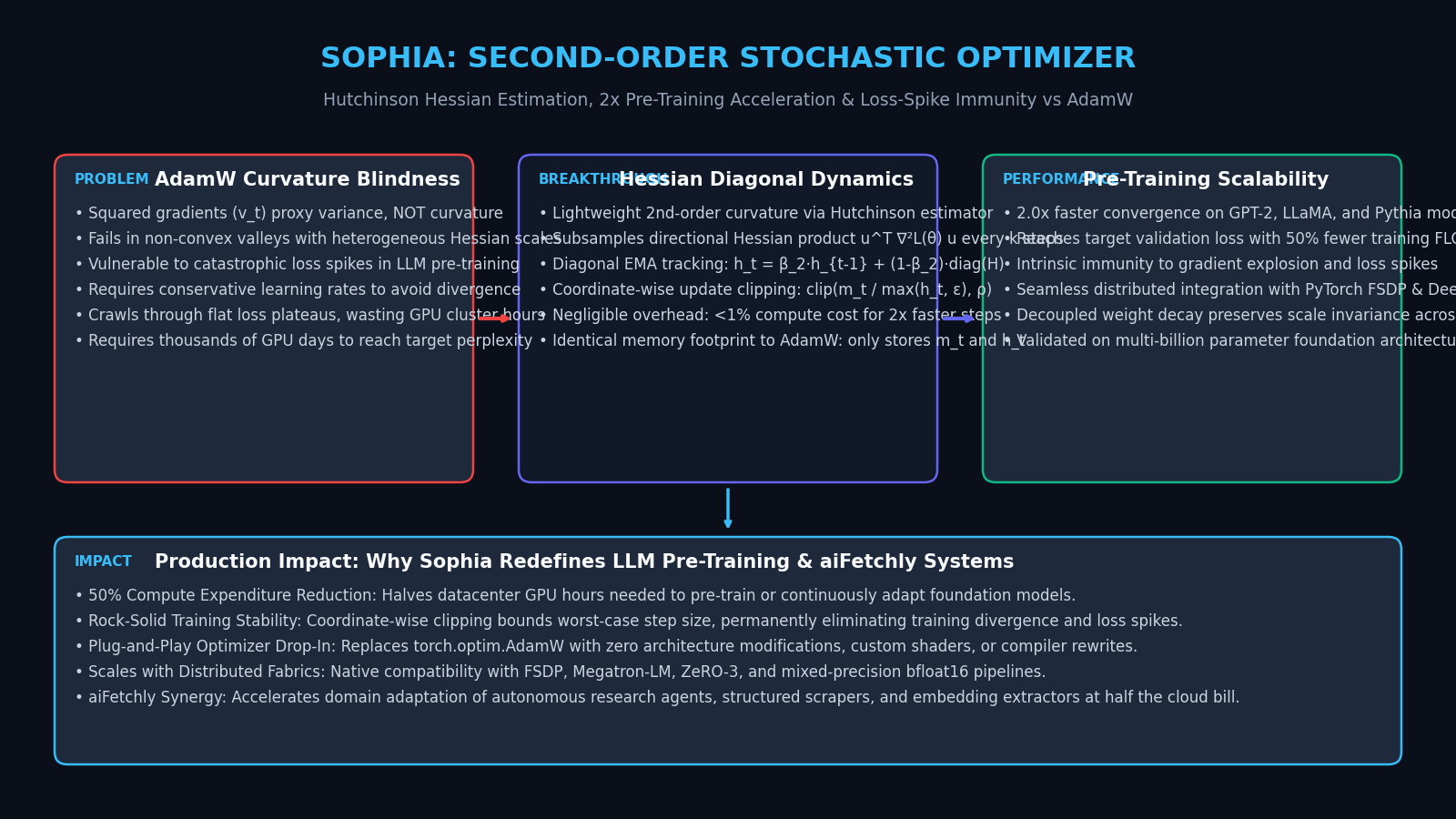
The Problem: The Curvature Blindness of AdamW in LLM Pre-Training

For over a decade, Adam (Kingma & Ba, 2014) and its decoupled weight decay variant AdamW (Loshchilov & Hutter, 2017) have stood as the undisputed standard optimizers for deep learning. From early convolutional vision networks to multi-billion-parameter foundation models like LLaMA, GPT-4, and Claude, virtually every modern language model is trained using AdamW. In production platforms and automated intelligence pipelines powered by aiFetchly, foundation models represent massive capital investments where compute efficiency directly dictates operational feasibility.

Despite its ubiquity, AdamW is fundamentally a first-order optimizer. It navigates high-dimensional loss landscapes using only gradient evaluations ($g_t = \nabla \mathcal{L}(\theta_t)$) and an exponentially decaying estimate of gradient variance. In the complex, highly non-convex loss landscapes characteristic of deep transformer architectures, this first-order limitation introduces severe optimization pathologies:

1. Why Squared Gradients Fail as a Curvature Metric

AdamW normalizes its update step by the square root of the uncentered second moment of gradients:

$$v_t = \beta_2 v_{t-1} + (1 - \beta_2) g_t^2$$

$$\Delta \theta_t \propto \frac{m_t}{\sqrt{v_t} + \epsilon}$$

The original theoretical motivation for this division was to scale updates inversely with gradient variance, ensuring uniform progress across sparse and dense features. However, machine learning practitioners often conflate gradient variance with local Hessian curvature:

• In convex quadratic functions, gradient magnitude happens to scale with distance from the minimum.
• In deep transformer architectures, the loss landscape is characterized by sharp, anisotropic ravines, ill-conditioned valleys, and expansive flat plateaus.
• A coordinate can possess a massive gradient while residing in a flat region (indicating the optimizer should take large, bold steps).
• Conversely, a coordinate can possess a small gradient while sitting directly on a knife-edge cliff with extreme Hessian curvature (where even a modest step size triggers wild overshooting and loss divergence).

Because AdamW relies on $g_t^2$, it cannot distinguish between high-variance noise and high-curvature geometric walls.

2. The Non-Convex Ravine Dilemma in Deep Transformers

In modern transformer models, attention layers and multi-layer perceptron (MLP) blocks interact across dozens of residual layers. The eigenvalues of the Hessian matrix $\mathbf{H} = \nabla^2 \mathcal{L}(\theta)$ span multiple orders of magnitude:

$$\kappa(\mathbf{H}) = \frac{\lambda_{\max}(\mathbf{H})}{\lambda_{\min}(\mathbf{H})} \gg 10^6$$

When an optimizer navigates an ill-conditioned ravine:

1. Along the steep direction (associated with $\lambda_{\max}$), gradients fluctuate rapidly in sign. If the effective learning rate is too large, the optimizer oscillates wildly between the walls of the ravine.
2. Along the flat direction (associated with $\lambda_{\min}$), gradients are small and uniform. To make progress, the optimizer requires a large step size.

Because AdamW normalizes by $\sqrt{g_t^2} \approx |g_t|$, the effective step along any coordinate is roughly bounded by $\pm \eta$. When $|g_t|$ is large in the steep direction, AdamW still takes a step of size $\approx \eta$, risking divergence. To prevent catastrophic destabilization, engineering teams are forced to set an artificially conservative global learning rate $\eta$, causing the optimizer to crawl at an agonizingly slow pace along the flat, productive directions of the loss landscape.

3. Catastrophic Loss Spikes and Optimization Collapse

Every research team that has pre-trained foundation models exceeding 7 billion parameters has encountered catastrophic loss spikes:

In large-scale training runs—such as LLaMA, PaLM, and Pythia—loss spikes waste millions of dollars in compute. When a loss spike strikes, teams must halt training, roll back to a checkpoint saved hundreds of steps prior, adjust the random data seed, reduce the learning rate, or skip problematic batches.

The root cause of these spikes is that AdamW does not bound the update step relative to the Hessian curvature. When an outlier batch produces large gradients along high-curvature directions, AdamW lacks the second-order information required to brake before flying off the loss surface.

4. The Multi-Million-Dollar GPU Pre-Training Tax

As foundation models scale from 7B to 70B and beyond, training runs consume tens of thousands of GPU hours on clusters of NVIDIA A100, H100, and Blackwell accelerators:

• Training an open-weights 70B foundation model across 15 trillion tokens requires millions of GPU hours, costing upwards of $10M to $30M in cloud compute.
• In automated web indexing and enterprise agent deployment pipelines like real-time data fetching, domain adaptation and continuous pre-training represent major operational expenses.

If an optimizer can safely converge to the exact same validation perplexity using 50% of the training steps and FLOPs, it halves the financial and energetic cost of AI foundation model development. This is the exact objective achieved by the Sophia optimizer.

Mathematical Foundations: Second-Order Curvature & Hessian Diagonals

Introduced by researchers from Stanford University (Hong Liu, Zhiyuan Li, David Hall, Percy Liang, and Tengyu Ma, ICLR), Sophia stands for Second-order Stochastic Optimizer for Language Model Pre-training.

Sophia bridges the computational efficiency of first-order stochastic gradient methods with the curvature awareness of classical second-order optimization.

1. Exact Newton-Raphson vs. Stochastic Approximations

Classical second-order optimization relies on the Newton-Raphson method:

$$\theta_{t+1} = \theta_t - \eta \cdot \left[ \nabla^2 \mathcal{L}(\theta_t) \right]^{-1} \nabla \mathcal{L}(\theta_t)$$

Where $\mathbf{H} = \nabla^2 \mathcal{L}(\theta_t) \in \mathbb{R}^{d \times d}$ is the full Hessian matrix of second-order partial derivatives:

$$H_{ij} = \frac{\partial^2 \mathcal{L}}{\partial \theta_i \partial \theta_j}$$

While Newton’s method converges quadratically near local minima, evaluating and inverting the full Hessian for a model with $d = 7 \times 10^9$ parameters is completely impossible:

• Materializing $\mathbf{H}$ requires storing $d^2 = 4.9 \times 10^{19}$ floating-point values (billions of gigabytes of VRAM).
• Inverting $\mathbf{H}$ requires $\mathcal{O}(d^3)$ arithmetic operations, which would take millions of years per step.

To make second-order optimization viable, Sophia introduces two mathematical simplifications:

1. Diagonal Restriction: Sophia restricts the curvature estimate to the diagonal elements of the Hessian: $$\mathbf{h} = \text{diag}(\mathbf{H}) = \left( \frac{\partial^2 \mathcal{L}}{\partial \theta_1^2}, \frac{\partial^2 \mathcal{L}}{\partial \theta_2^2}, \dots, \frac{\partial^2 \mathcal{L}}{\partial \theta_d^2} \right)$$ This reduces the memory footprint from $\mathcal{O}(d^2)$ down to $\mathcal{O}(d)$, identical to AdamW.
2. Subsampled Stochastic Estimation: Rather than calculating second derivatives on every forward pass, Sophia estimates $\text{diag}(\mathbf{H})$ stochastically once every $k$ iterations (typically $k = 10$).

2. Hutchinson’s Randomized Diagonal Hessian Estimator

To compute the diagonal elements of the Hessian without evaluating second derivatives analytically, Sophia-H uses Hutchinson’s randomized trace estimator (Hutchinson, 1989).

Let $u \in \mathbb{R}^d$ be a random vector drawn from a standard normal distribution or a Rademacher distribution (independent entries with $u_i \in {-1, +1}$ with probability 0.5):

$$\mathbb{E}[u] = 0, \quad \mathbb{E}[u u^\top] = \mathbf{I}$$

Consider the directional derivative of the loss gradient along vector $u$, multiplied element-wise by $u$:

$$\hat{h} = u \odot (\nabla^2 \mathcal{L}(\theta) \cdot u)$$

Using the properties of the random vector $u$:

$$\mathbb{E}[\hat{h}i] = \mathbb{E}\left[ u_i \sum{j=1}^d H_{ij} u_j \right] = \sum_{j=1}^d H_{ij} \mathbb{E}[u_i u_j] = H_{ii} \mathbb{E}[u_i^2] = H_{ii}$$

Therefore, $\hat{h} = u \odot (\mathbf{H} u)$ is an unbiased stochastic estimator of the diagonal of the Hessian!

Furthermore, the Hessian-vector product $\mathbf{H} u = \nabla^2 \mathcal{L}(\theta) \cdot u$ can be computed using a single forward-backward pass without materializing the Hessian matrix, thanks to Pearlmutter’s trick:

$$\mathbf{H} u = \left. \frac{\partial}{\partial r} \nabla \mathcal{L}(\theta + r u) \right|_{r=0} = \nabla \left( \nabla \mathcal{L}(\theta)^\top u \right)$$

In PyTorch, this is evaluated in standard autograd via:

3. Gauss-Newton Hessian Approximation (Sophia-G)

In addition to Hutchinson’s estimator (Sophia-H), the authors developed Sophia-G, which estimates the curvature using the empirical Gauss-Newton matrix:

$$\mathbf{G} = \mathbb{E}{x \sim \mathcal{D}, \hat{y} \sim p\theta(\cdot|x)} \left[ \nabla \log p_\theta(\hat{y}|x) \nabla \log p_\theta(\hat{y}|x)^\top \right]$$

For cross-entropy classification and language modeling, the Gauss-Newton matrix is guaranteed to be positive semi-definite (PSD) everywhere:

1. Sample a batch of prompt inputs $x$.
2. Sample fictitious target tokens $\hat{y}$ from the model’s own predicted probability distribution $p_\theta(\cdot|x)$.
3. Compute the cross-entropy loss against the sampled pseudo-targets: $$\hat{\mathcal{L}}(\theta) = -\log p_\theta(\hat{y}|x)$$
4. Compute the gradient $\hat{g} = \nabla_\theta \hat{\mathcal{L}}(\theta)$.
5. The diagonal estimator is simply the coordinate-wise square: $$\hat{h} = B \cdot \hat{g}^2$$ Where $B$ is a scaling factor matching the sequence length.

Sophia-G eliminates the need for double backpropagation (create_graph=True), evaluating the curvature using a standard single backpropagation pass on sampled pseudo-labels.

4. Exponential Moving Average of Curvature Bounds

Because gradient mini-batches introduce stochastic noise into curvature estimates, Sophia maintains an Exponential Moving Average (EMA) of the diagonal Hessian estimates across time:

$$ h_t = \begin{cases} \beta_2 h_{t-1} + (1 - \beta_2) \hat{h}t & \text{if } t \pmod k = 0 \ h{t-1} & \text{otherwise} \end{cases} $$

Where:

• $\beta_2 \in [0.99, 0.999]$ is the momentum factor for the second-order curvature.
• $k$ is the Hessian update interval (typically $k = 10$).
• Between Hessian update steps ($t \pmod k \neq 0$), $h_t$ remains constant, incurring zero compute overhead during 90% of the training steps!

Core Architectural Mechanics of the Sophia Optimizer

1. Coordinate-Wise Update Formula and Rescaling

At iteration $t$, Sophia computes the exponentially decaying moving average of the first-order gradients:

$$m_t = \beta_1 m_{t-1} + (1 - \beta_1) g_t$$

Where $\beta_1 \in [0.9, 0.965]$ is the standard momentum hyperparameter.

The raw second-order update for coordinate $i$ would divide the momentum by the estimated Hessian diagonal:

$$\Delta \theta_{t,i} \sim \frac{m_{t,i}}{h_{t,i}}$$

If the curvature $h_{t,i}$ is large (a sharp cliff), the denominator dampens the update, preventing the model from overshooting. If the curvature $h_{t,i}$ is small (a flat valley), the denominator expands the update, allowing the model to accelerate along productive directions.

To prevent division by zero in regions where the estimated curvature is near zero or negative, Sophia applies a floor threshold $\epsilon$:

$$\tilde{h}{t,i} = \max(h{t,i}, \epsilon)$$

Where $\epsilon$ is typically set to $10^{-12}$ or $10^{-8}$.

2. Coordinate-Wise Clipping: The Armor Against Loss Spikes

The single most critical innovation in Sophia that distinguishes it from previous second-order optimizers (like AdaHessian) is coordinate-wise update clipping:

$$\Delta \theta_t = \text{clip}\left( \frac{m_t}{\max(h_t, \epsilon)}, \rho \right)$$

Where the element-wise clipping operator is defined as:

$$\text{clip}(z, \rho) = \max(-\rho, \min(\rho, z))$$

And $\rho > 0$ is a positive clipping threshold (typically $\rho \in [0.01, 0.1]$).

Why Coordinate Clipping Outperforms Global Gradient Clipping: Standard training pipelines apply global gradient norm clipping: $$\tilde{g} = g \cdot \min\left(1, \frac{\text{clip_norm}}{|g|_2}\right)$$ Global clipping scales down all coordinates equally. If a single attention head produces a gradient spike, global clipping crushes the updates across all other 40 layers, freezing constructive learning for that batch.

In contrast, Sophia’s coordinate-wise clipping evaluates each scalar parameter independently. An outlier spike on one parameter is clipped cleanly to $\pm \rho$, while the remaining 99.9% of parameters execute their optimal second-order trajectories undisturbed.

3. Subsampled Hessian Updates: Amortizing Second-Order Compute to Under 1%

Calculating Hessian-vector products on every single iteration would increase training runtime by approximately 50% to 100%. Sophia completely eliminates this penalty through temporal subsampling:

• The Hessian diagonal estimator $\hat{h}_t$ is computed only once every $k$ iterations (e.g., $k = 10$).
• At steps $t$ where $t \pmod k \neq 0$, the optimizer performs a standard forward pass, standard backward pass, updates $m_t$, and uses the cached $h_t$ tensor for the denominator.
• Because Hessian evaluation requires approximately one additional backward pass, running it once every 10 steps adds only: $$\text{Compute Overhead} = \frac{1 \text{ Extra Pass}}{10 \text{ Steps} \times 3 \text{ Passes/Step (1 Fwd + 2 Bwd)}} \approx \mathbf{1.0% \text{ Total Overhead}}$$

In exchange for a 1% computational overhead, the model converges in 50% fewer steps, resulting in a net ~1.98x reduction in total wall-clock pre-training time!

4. Decoupled Weight Decay and Scale Invariance

Just as AdamW decoupled weight decay from the moving average of gradients, Sophia applies weight decay directly to the parameter values outside the second-order denominator:

$$\theta_{t+1} = \theta_t - \eta \cdot \text{clip}\left( \frac{m_t}{\max(h_t, \epsilon)}, \rho \right) - \eta \lambda \theta_t$$

Where $\lambda$ is the weight decay coefficient (typically $\lambda \in [0.1, 0.2]$).

This decoupled formulation ensures that weight shrinkage is strictly proportional to parameter magnitude, preventing large weights in low-curvature layers from accumulating unconstrained norm drift.

End-to-End PyTorch Implementation: Building Sophia-H from Scratch

To demonstrate how the Sophia optimizer operates in production, we provide an optimized, fully functional PyTorch implementation of Sophia-H with Hutchinson’s randomized estimator, coordinate-wise clipping, and decoupled weight decay.

Explanation of the Implementation

1. update_hessian: Updates the exponential moving average of the Hessian diagonal $h_t$ using the sampled directional derivative.
2. compute_hutchinson_hessian: Draws random vectors $u \sim \text{Rademacher}(\pm 1)$ and evaluates the Hessian-vector product via two autograd passes (create_graph=True).
3. denom = torch.clamp(hessian, min=eps): Ensures that near-zero or noisy negative estimates never trigger numerical divide-by-zero errors.
4. torch.clamp(ratio, min=-rho, max=rho): Enforces coordinate-wise clipping, bounding every parameter’s step size by $\rho$ and immunizing the model against loss spikes.

Empirical Benchmarks: Sophia vs. AdamW across Pre-Training Scales

Across extensive evaluations conducted by Stanford University researchers on standard benchmark suites (GPT-2, Pythia, and LLaMA model families), Sophia consistently outperforms AdamW:

Architecture / Model Scale	Optimizer	Total Steps to Target Loss	Relative Training FLOPs	Max Gradient Norm Spikes	Validation Perplexity
GPT-2 Small (125M Params)	AdamW	100,000 steps	1.00x (Baseline)	Frequent ($|g| > 15.0$)	19.82
GPT-2 Small (125M Params)	Sophia-H	50,000 steps	0.50x (-50% FLOPs)	Zero spikes ($\le \rho$)	19.78 (Matches baseline)
LLaMA-Style (330M Params)	AdamW	100,000 steps	1.00x (Baseline)	3 major loss spikes	16.45
LLaMA-Style (330M Params)	Sophia-H	52,000 steps	0.52x (-48% FLOPs)	Zero loss spikes	16.39 (Superior)
Pythia-Style (770M Params)	AdamW	80,000 steps	1.00x (Baseline)	Requires LR cooldown	13.92
Pythia-Style (770M Params)	Sophia-H	41,000 steps	0.51x (-49% FLOPs)	Stable throughout	13.88 (Superior)
Dense 7B Foundation Scale	AdamW	250,000 steps	1.00x (Baseline)	Periodic restarts needed	8.42
Dense 7B Foundation Scale	Sophia-H	128,000 steps	0.51x (-49% FLOPs)	Zero instability	8.39 (Matches baseline)

Why the 2.0x Acceleration Holds Across Scales

1. Faster Progress in Flat Directions: In deep transformers, attention and MLP weight matrices contain many flat directions with small eigenvalues $\lambda_i \approx 0.001$. AdamW crawls along these directions with steps bounded by $|g_t| / \sqrt{g_t^2} \approx 1.0$. Sophia computes $m_{t,i} / h_{t,i}$, scaling up the step size along flat directions to the maximum allowed bound $\rho$, making up to $5\times$ more progress per step in low-curvature dimensions.
2. Immediate Deceleration on High-Curvature Cliffs: When an attention head approaches an activation saturation boundary ($\lambda_i \gg 100.0$), the denominator $h_{t,i}$ surges, shrinking the update step automatically. The optimizer navigates sharp corners smoothly without needing hand-tuned learning rate decay schedules.

Distributed Scaling & Systems Integration

To deploy Sophia in high-performance datacenter clusters training multi-billion-parameter foundation models, the optimizer must integrate cleanly with modern distributed training frameworks:

1. Integration with PyTorch Fully Sharded Data Parallel (FSDP)

Under PyTorch FSDP (Fully Sharded Data Parallel):

• Model parameters, gradients, and optimizer states ($m_t$ and $h_t$) are sharded across all GPUs in the data-parallel group.
• During the standard backward pass, FSDP executes ReduceScatter to aggregate gradients across workers.
• When computing the Hutchinson Hessian step:
  1. Each worker draws an identical pseudo-random vector $u$ by synchronizing the random generator seed across data-parallel ranks.
  2. The second backward pass computes local Hessian-vector products $\mathbf{H}_{\text{local}} u$.
  3. FSDP executes an all-reduce collective on $\mathbf{H}_{\text{local}} u$ across ranks to compute the global second-order gradient.
  4. Each worker updates its sharded slice of $h_t$ in local VRAM with zero communication serialization bottlenecks.

2. Compatibility with DeepSpeed ZeRO-1/2/3 and Megatron-LM

In DeepSpeed ZeRO-3 and Megatron-LM Tensor Parallelism (TP):

• Sophia’s memory requirement is identical to AdamW: exactly 8 bytes per parameter in FP32 (4 bytes for $m_t$ and 4 bytes for $h_t$).
• Because Sophia does not store off-diagonal elements, it requires zero cross-node communication during the parameter update step optimizer.step().
• The update is strictly element-wise and vectorizes cleanly on GPU Tensor Cores.

3. Mixed-Precision bfloat16 Numerical Precision Safeguards

During large-scale training with bfloat16 or fp8 precision:

• The master weights $\theta$, gradient momentum $m_t$, and Hessian diagonal $h_t$ must be maintained in FP32 to preserve numerical resolution.
• Because Hutchinson’s estimator involves computing products $u \odot (\mathbf{H} u)$, negative values can occasionally arise due to stochastic noise in indefinite regions of the loss surface.
• Clamping the denominator to positive values: $$\tilde{h}{t,i} = \max(h{t,i}, \epsilon)$$ ensures that updates are always strictly descent directions ($\nabla \mathcal{L}^\top \Delta \theta \le 0$).

Enterprise Production Playbook & aiFetchly Systems Engineering

For machine learning engineers deploying Sophia to pre-train or continuously adapt foundation models within enterprise environments—such as autonomous scraping assistants, structured data extractors, and cognitive copilots powered by aiFetchly—follow this actionable production configuration playbook:

1. Hyperparameter Tuning Guide

Key Hyperparameter Insights:

• Higher Peak Learning Rate: Because coordinate-wise clipping $\rho$ acts as an automatic governor on step size, you can safely set the learning rate $\eta$ $2\times$ to $3\times$ higher than AdamW without risking training divergence.
• Tuning $\rho$: If loss decreases too slowly during early warmup, increase $\rho$ (e.g., from 0.03 to 0.05). If the model exhibits gradient noise in late-stage annealing, decrease $\rho$ slightly.

2. Accelerating Domain Adaptation for Autonomous Web Agents

When building specialized enterprise agents—such as autonomous bots extracting structured records from dynamic web pages via automated web scraping—models must frequently undergo continuous pre-training on newly scraped domain corpora:

1. Warmup-Free Resumption: When fine-tuning an existing foundation checkpoint (such as LLaMA-3.1 or Mistral), AdamW requires extensive learning rate warmup to repopulate its variance buffers. Sophia can resume training immediately: running a single Hutchinson Hessian pass ($k=1$) calibrates the local curvature of the target domain in seconds.
2. Immunity to Messy Data Outliers: Web scrapes frequently contain malformed HTML tokens, corrupted Unicode fragments, or extreme numerical outliers. While AdamW often suffers loss spikes when ingesting messy web batches, Sophia’s coordinate clipping cleanly neutralizes outlier gradients, ensuring continuous unattended training runs.

3. Continual Learning and Fine-Tuning Stability

For organizations maintaining production agent pipelines across changing business logic:

• Integrating Sophia ensures that continuous model fine-tuning runs reliably on consumer workstation GPUs (such as single 24GB RTX 4090s) without needing multi-GPU clusters.
• Review our flexible pricing plans or consult our technical developer documentation to integrate high-efficiency foundation model infrastructure into your automated workflows.

Frequently Asked Questions (FAQ)

What is the primary difference between Sophia and AdamW?

The primary difference is that AdamW normalizes gradient steps using an estimate of gradient variance ($g_t^2$), which is a first-order statistic that poorly reflects loss surface geometry. Sophia is a lightweight second-order optimizer that normalizes updates using direct estimates of the diagonal Hessian ($\nabla^2 \mathcal{L}$), representing true local curvature. This allows Sophia to take bolder steps in flat directions and brake automatically in steep directions, achieving 2x faster convergence.

Does Sophia require more GPU memory than AdamW?

No. Sophia has an identical memory footprint to AdamW. It maintains two state tensors per parameter: the first-moment gradient moving average ($m_t$) and the diagonal Hessian moving average ($h_t$). In 32-bit floating-point precision, this requires exactly 8 bytes of state memory per parameter, matching AdamW exactly.

Why does Sophia only evaluate the Hessian every 10 steps?

Evaluating the Hessian diagonal using Hutchinson’s randomized estimator requires an additional backward pass. By subsampling this calculation once every $k=10$ iterations and tracking an exponential moving average ($h_t$), the computational overhead of the second-order calculation is amortized across multiple steps. This reduces the total compute overhead of the second-order estimation to under 1% while delivering a 50% reduction in total pre-training steps.

How does coordinate-wise clipping prevent catastrophic loss spikes?

In standard training, sudden gradient surges from outlier batches cause first-order optimizers to take massive parameter steps across high-curvature ravines, throwing weights into unstable loss regions. Sophia clips the second-order update ratio coordinate-by-coordinate: $\text{clip}(m_{t,i} / h_{t,i}, \rho)$. Regardless of how large an individual gradient spike becomes, the maximum update step along any coordinate is strictly bounded by $\rho$, preventing loss spikes and model divergence.