SigLIP Architecture: Sigmoid Loss Vision-Language Models
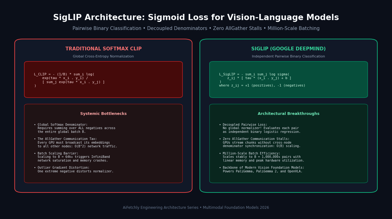
The Problem: The All-Gather Communication Wall in Softmax CLIP
In modern multimodal artificial intelligence, visual grounding engines, and autonomous web extraction platforms like AiFetchly, aligning visual pixels with human language representations is foundational. For years, the undisputed industry standard for multimodal pre-training was CLIP (Contrastive Language-Image Pre-Training), introduced by OpenAI (Radford et al., 2021).
CLIP trains a dual-encoder architecture—a Vision Transformer (ViT) and a Text Transformer—by projecting images and text into a shared latent embedding space. To learn joint representations, CLIP minimizes a symmetric Softmax Cross-Entropy Loss over a batch of $B$ paired image-text examples:
$$\mathcal{L}{\text{CLIP}} = -\frac{1}{2B} \sum{i=1}^B \left( \log \frac{\exp(\tau \cdot \mathbf{x}_i^\top \mathbf{y}i)}{\sum{j=1}^B \exp(\tau \cdot \mathbf{x}_i^\top \mathbf{y}_j)} + \log \frac{\exp(\tau \cdot \mathbf{y}_i^\top \mathbf{x}i)}{\sum{j=1}^B \exp(\tau \cdot \mathbf{y}_i^\top \mathbf{x}_j)} \right)$$
Where $\mathbf{x}_i$ is the normalized image embedding, $\mathbf{y}_j$ is the normalized text embedding, and $\tau$ is a learned temperature parameter.
While CLIP achieved historic breakthroughs in zero-shot image classification and image-text retrieval, scaling CLIP to modern high-performance GPU clusters revealed three severe architectural bottlenecks:
1. The Global Softmax Denominator and All-Gather Synchronization Stalls
Notice the denominator in the CLIP loss: $$\sum_{j=1}^B \exp(\tau \cdot \mathbf{x}_i^\top \mathbf{y}_j)$$ To compute the probability distribution over all competing candidates, the softmax operator requires summing across every negative text example in the entire global batch $B$:
- In distributed multi-node training across 64, 128, or 512 GPUs, each GPU holds only a small micro-batch of images and captions.
- Before computing the softmax loss, every worker node must execute a blocking collective communication primitive:
torch.distributed.all_gather. - All GPUs must broadcast their local embedding vectors across the cluster’s network fabric to reconstruct the full $B \times B$ similarity matrix.
- As distributed systems scale, network communication overhead explodes quadratically: $$\mathcal{O}(B^2) \quad \text{in inter-node data exchange}$$
- GPUs spend massive computational cycles idling in network synchronization barriers waiting for InfiniBand or Ethernet packets, crippling scaling efficiency.
2. The Extreme Imbalance Scaling Ceiling
Contrastive learning thrives on massive negative candidate pools: larger batches expose the model to harder negative distractors, refining semantic boundaries.
- However, because CLIP’s memory footprint for the similarity matrix scales as $\mathcal{O}(B^2)$, pushing global batch sizes beyond 32,768 or 65,536 tokens exhausts GPU High-Bandwidth Memory (HBM).
- When developers attempt to save memory via gradient checkpointing or multi-stage gathering, communication latency dominates execution time, capping maximum practical batch sizes.
3. Outlier Distortions in Coupled Normalization
Because softmax enforces a strict probability distribution that must sum to 1.0:
- Every image-text pair’s gradient is directly coupled to every other candidate in the batch.
- If a noisy web-scraped dataset contains a severely mislabeled or outlier caption, its massive exponentiated dot-product artificially suppresses the denominator for all other valid pairs in the batch, destabilizing optimization trajectories.
The Solution: SigLIP’s Decoupled Sigmoid Loss Formulation
To dismantle the communication bottleneck, researchers at Google DeepMind (Zhai et al., ICCV 2023) introduced SigLIP (Sigmoid Loss for Language-Image Pre-Training).
SigLIP makes a deceptively simple yet mathematically profound conceptual leap: replace the global multi-class softmax normalizer with independent pairwise binary classification.
The Mathematical Formulation of SigLIP
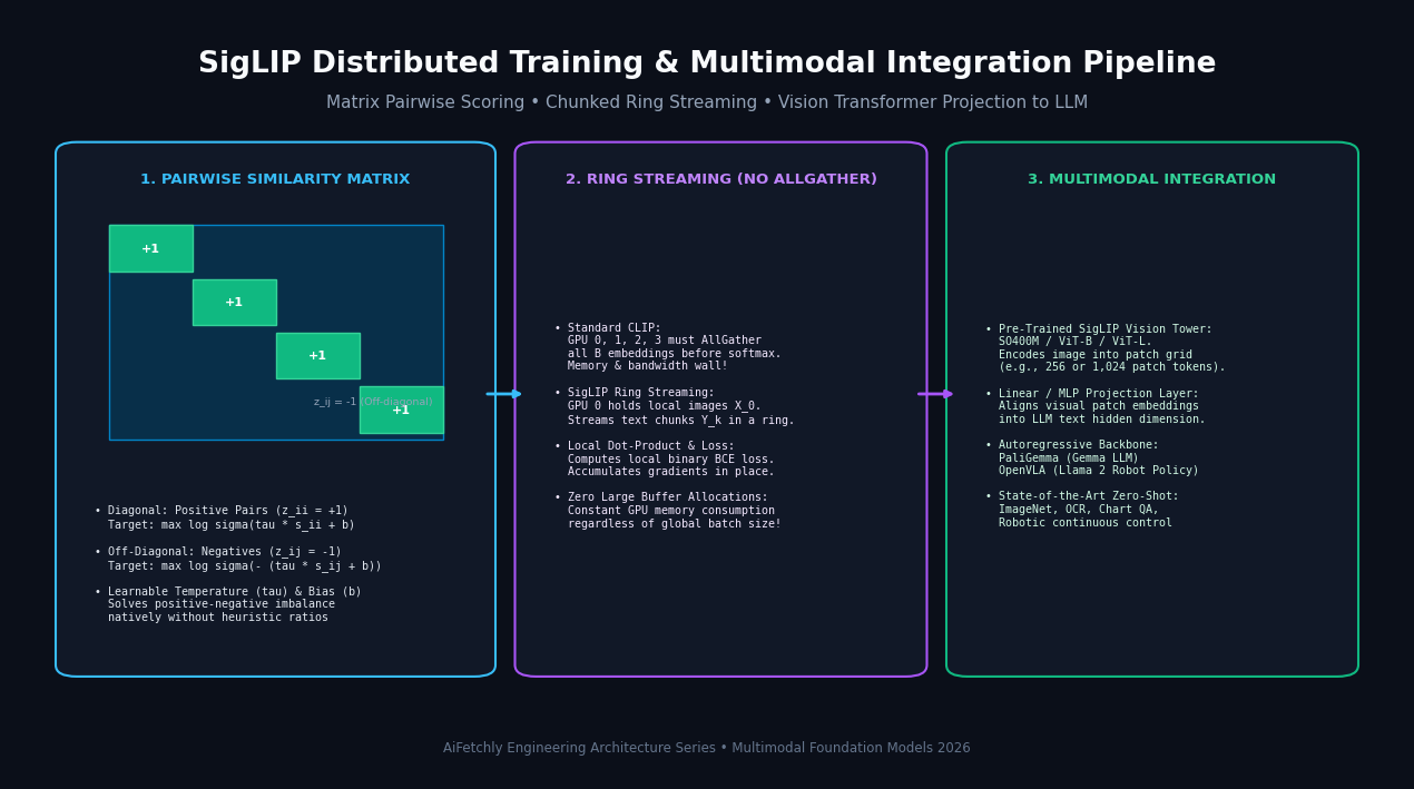
Instead of asking “Which text out of the $B$ candidates matches this image?” (a multinomial choice), SigLIP asks $B^2$ independent binary questions: “Does image $i$ match text $j$?” (yes or no).
The SigLIP loss is defined as:
$$\mathcal{L}{\text{SigLIP}} = - \frac{1}{B} \sum{i=1}^B \sum_{j=1}^B \log \sigma \left( z_{ij} \cdot \left[ \tau (\mathbf{x}_i^\top \mathbf{y}_j) + b \right] \right)$$
Where:
- $\sigma(u) = \frac{1}{1 + e^{-u}}$ is the standard sigmoid logistic function.
- $z_{ij} \in {-1, +1}$ is the binary ground-truth label: $$z_{ij} = \begin{cases} +1 & \text{if } i = j \quad (\text{positive matched pair}) \ -1 & \text{if } i \neq j \quad (\text{negative unmatched pair}) \end{cases}$$
- $\tau$ is a learnable temperature scale parameter (initialized around $\log 10$).
- $b$ is a learnable bias parameter (initialized around $-10$).
The Role of the Learnable Bias ($b$)
In a batch of size $B = 32,768$, there are exactly $B$ positive pairs on the diagonal and $B^2 - B \approx 1.07 \times 10^9$ negative pairs off the diagonal. The ratio of positives to negatives is roughly $1 : B$.
In naive binary classification, such an overwhelming negative skew causes gradients to collapse toward predicting negative for everything. The learnable scalar bias $b$ solves this natively:
- By initializing $b$ to a large negative value (e.g., $-10$), the model begins training with the prior assumption that arbitrary pairs are overwhelmingly non-matching: $$\sigma(b) = \frac{1}{1 + e^{10}} \approx 0.000045$$
- The network does not waste gradient energy pushing negative probabilities to zero; it focuses parameters on detecting positive semantic alignments.
The Systems Mechanics: Ring Chunk Streaming and All-Gather Elimination
The transformative operational advantage of SigLIP lies in its distributed memory layout. Because SigLIP decomposes into an unnormalized sum of independent pairwise cross-entropies:
$$\mathcal{L}{\text{SigLIP}} = \sum{i} \sum_{j} \ell(x_i, y_j)$$
There is no global denominator requiring simultaneous visibility of the entire batch.
Ring Chunk Streaming (Zero All-Gather Stalls)
Instead of performing an expensive global AllGather of all embeddings:
- Each GPU processes its local batch of images $X_{\text{local}}$ and texts $Y_{\text{local}}$.
- The GPU calculates the binary loss for local positive pairs ($z_{ii} = +1$) and local negative pairs.
- To compare against non-local negatives, the GPU cluster organizes into a Ring Topology:
- GPU $k$ retains its local image embeddings in High-Bandwidth Memory (HBM).
- In the background, GPU $k$ streams its small text embedding buffer to GPU $k+1$ using asynchronous non-blocking point-to-point transfers (
P2Ppeer-to-peer ring communication). - While the next text chunk is in-flight across the network, the GPU computes matrix multiplications against the current text chunk and accumulates loss gradients in place.
- Memory Complexity: GPU memory usage remains strictly bounded by the local chunk size, completely decoupled from the global batch size $B$.
- Communication Complexity: Communication drops from quadratic all-to-all broadcasts to lightweight linear streaming: $$\mathcal{O}(B) \quad \text{linear communication overhead}$$
This allows distributed teams to train models with effective batch sizes of 1,000,000+ pairs without running out of VRAM or hitting network bandwidth walls.
Implementation: PyTorch Numerical Loss & Hugging Face Usage
To understand the mechanics, let us first implement the exact numerical SigLIP loss in PyTorch, followed by loading and running a pre-trained SigLIP vision tower via the Hugging Face Transformers library.
import torch
import torch.nn as nn
import torch.nn.functional as F
from PIL import Image
from transformers import AutoProcessor, AutoModel

# 1. Mathematical PyTorch Implementation of SigLIP Loss
class SigLIPLoss(nn.Module):
    def __init__(self, init_tau: float = 10.0, init_b: float = -10.0):
        super().__init__()
        # Learnable temperature and bias parameters
        self.log_tau = nn.Parameter(torch.log(torch.tensor(init_tau)))
        self.bias = nn.Parameter(torch.tensor(init_b))

    def forward(self, image_embeds: torch.Tensor, text_embeds: torch.Tensor) -> torch.Tensor:
        # Normalize embeddings to unit hypersphere
        image_embeds = F.normalize(image_embeds, p=2, dim=-1)
        text_embeds = F.normalize(text_embeds, p=2, dim=-1)

        batch_size = image_embeds.shape[0]
        tau = torch.exp(self.log_tau)

        # Compute pairwise dot-product similarity matrix: [B, B]
        logits = tau * torch.matmul(image_embeds, text_embeds.T) + self.bias

        # Construct ground truth labels: +1 along diagonal, -1 off-diagonal
        # In PyTorch: log(sigma(u)) = -F.softplus(-u)
        labels = 2.0 * torch.eye(batch_size, device=image_embeds.device) - 1.0

        # Log-sigmoid binary loss: -log sigma(z_ij * logits) = softplus(-z_ij * logits)
        loss = F.softplus(-labels * logits).sum() / batch_size
        return loss

# 2. Production Inference with Google Pre-Trained SigLIP (SO400M)
def run_siglip_zero_shot():
    model_name = "google/siglip-so400m-patch14-384"
    print(f"Loading {model_name}...")

    processor = AutoProcessor.from_pretrained(model_name)
    model = AutoModel.from_pretrained(model_name)
    model.eval()

    # Create dummy RGB image (simulating e-commerce product extraction)
    dummy_image = Image.new("RGB", (384, 384), color=(73, 109, 137))
    candidate_labels = [
        "a screenshot of a software pricing dashboard",
        "a photo of an outdoor mountain landscape",
        "an architecture diagram of a neural network",
        "a modern smartphone on a wooden desk"
    ]

    # Preprocess inputs
    inputs = processor(
        text=candidate_labels,
        images=dummy_image,
        padding="max_length",
        return_tensors="pt"
    )

    with torch.no_grad():
        outputs = model(**inputs)
        logits_per_image = outputs.logits_per_image

        # In SigLIP, probabilities are computed via sigmoid per candidate, NOT softmax!
        probs = torch.sigmoid(logits_per_image).squeeze().tolist()

    print("\n--- SigLIP Pairwise Binary Probabilities ---")
    for label, prob in zip(candidate_labels, probs):
        print(f"Candidate: '{label}' -> Probability: {prob:.4f}")

if __name__ == "__main__":
    # Test loss function with synthetic representations
    criterion = SigLIPLoss()
    synth_images = torch.randn(16, 512)
    synth_texts = torch.randn(16, 512)
    computed_loss = criterion(synth_images, synth_texts)
    print(f"Calculated Synthetic SigLIP Loss: {computed_loss.item():.4f}")

    # Run Hugging Face model
run_siglip_zero_shot() Architectural Comparison: SigLIP vs. CLIP vs. Modern Multimodal Vision Towers
To understand why modern foundation models have shifted away from classic CLIP, consider how SigLIP compares against other visual representations:
| Feature Dimension | OpenAI CLIP (2021) | OpenCLIP / DFN (2023) | Google SigLIP (2023/2024) | Meta DINOv2 (2023) |
|---|---|---|---|---|
| Objective Function | Symmetric Softmax Cross-Entropy | Filtered Softmax Contrastive | Pairwise Sigmoid Binary Loss | Self-Supervised DINO / iBOT |
| Normalizer Scope | Global batch denominator | Global batch denominator | Decoupled (No global sum) | Patch-level cluster centers |
| Communication Overhead | $\mathcal{O}(B^2)$ AllGather sync stalls | $\mathcal{O}(B^2)$ AllGather sync stalls | $\mathcal{O}(B)$ Ring Chunk Streaming | Local GPU gradient all-reduce |
| Learned Parameters | Scale $\tau$ only | Scale $\tau$ only | Scale $\tau$ + Learned Bias $b$ | Centering & temperature heads |
| Max Practical Batch Size | 32k to 64k pairs | 64k to 128k pairs | 1,000,000+ pairs | Standard batch sizes (2k-4k) |
| Zero-Shot ImageNet Top-1 | 75.4% (ViT-L/14) | 79.2% (ViT-H/14) | 83.1% (ViT-SO400M) | Linear probe only (86.5%) |
| Modern Downstream Models | Stable Diffusion 1.5/2.1 | SDXL / Flux | PaliGemma, Gemma-2, OpenVLA | Depth, Segmentation, OpenVLA |
While self-supervised models like DINOv2 excel at dense pixel-level spatial features (depth estimation and dense segmentation), SigLIP represents the premier open visual backbone for connecting vision to language, outperforming CLIP across ImageNet zero-shot, COCO retrieval, and visual question answering.
Downstream Integration: Powering PaliGemma, PaliGemma 2, and OpenVLA
Because SigLIP produces dense visual patch tokens with exceptional semantic grounding, frontier AI engineering has adopted pre-trained SigLIP vision towers as the default visual encoder for autoregressive Vision-Language Models (VLMs):
1. Google PaliGemma and PaliGemma 2
Google DeepMind’s open foundation VLM, PaliGemma, directly connects a pre-trained SigLIP-SO400M vision tower with a Gemma autoregressive language model:
- The SigLIP encoder takes a 448x448 or 896x896 image, splits it into 14x14 pixel patches, and outputs a grid of dense visual tokens (e.g., 1,024 tokens).
- A linear projection layer aligns the SigLIP feature dimension (1,152) into Gemma’s text embedding dimension (2,048).
- The visual tokens are prepended directly to the text token sequence, allowing the model to perform OCR, bounding box object detection, document parsing, and complex visual reasoning in a single autoregressive forward pass.
2. OpenVLA Robotics Foundation Model
In physical embodied AI, the OpenVLA generalist robot policy (Stanford, Berkeley, DeepMind) combines a SigLIP vision encoder with DINOv2:
- DINOv2 provides structural spatial geometry (object depths, edges, and distances).
- SigLIP provides high-level semantic language alignment (understanding instructions like “pick up the red mug next to the laptop”).
- Together, they feed visual features into a 7B parameter policy backbone that predicts continuous 7-DoF robot arm actions at 10Hz.
3. Production Best Practices for Multimodal Data Extraction
In high-frequency extraction engines like AiFetchly:
- When performing document parsing or screen understanding, replace fragile OCR pipelines with compact SigLIP-based vision encoders.
- Because SigLIP operates on binary sigmoid probabilities, multi-label zero-shot classification (e.g., identifying multiple UI widgets present in a single screenshot) does not require arbitrary threshold hacking: each candidate label is evaluated independently against a calibrated sigmoid probability.
By discarding the legacy softmax denominator and embracing pairwise binary classification, SigLIP demonstrates how principled mathematical reparameterization can unlock exponential efficiency gains across modern artificial intelligence infrastructure.