rwkvlinear-attentionstate-space-modelsllm-architecturetutorial

RWKV-v6 Architecture: Attention-Free Linear Transformers

September 22, 2026

RWKV-v6 Architecture: Linear Attention, Matrix Recurrence, and Constant Memory Inference

The Problem: The Quadratic Wall and KV Cache Bloat of Softmax Attention

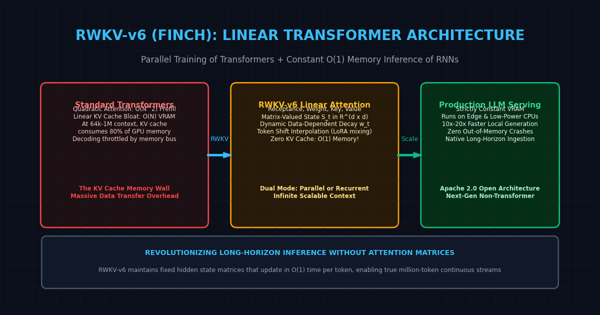
In high-throughput enterprise pipelines and autonomous monitoring systems like AiFetchly, deploying standard transformer models for continuous, long-horizon generation exposes two fundamental scaling bottlenecks:

1. The Quadratic Prefill Bottleneck ($O(N^2)$)

Standard Multi-Head Attention (MHA) calculates pairwise dot products across every token in the sequence:

$$\text{Attention}(\mathbf{Q}, \mathbf{K}, \mathbf{V}) = \text{Softmax}\left(\frac{\mathbf{Q} \mathbf{K}^T}{\sqrt{d_k}}\right) \mathbf{V}$$

As prompt context expands to 64,000, 128,000, or 1,000,000 tokens, computing the $N \times N$ attention matrix requires quadratic computational FLOPs and introduces severe Time-to-First-Token (TTFT) latency spikes.

2. The Linear KV Cache Memory Wall ($O(N)$)

During autoregressive generation, a transformer stores the Key ($\mathbf{K}$) and Value ($\mathbf{V}$) activation tensors for every historical token in High Bandwidth Memory (HBM). For a 70B parameter model serving a 100,000-token stream, the KV cache alone consumes over 80GB of GPU VRAM—exceeding the memory capacity of an entire NVIDIA H100 GPU before accounting for model weights.

Furthermore, decoding is memory-bandwidth bound: streaming gigabytes of past KV vectors across the memory bus to generate a single new token slows generation speeds to a crawl.

Historically, classical Recurrent Neural Networks (RNNs, like LSTMs and GRUs) offered constant $O(1)$ inference memory, but they could not scale: they suffered from catastrophic forgetting over long sequences and could not be parallelized across GPU Tensor Cores during training.

The Architecture: Receptance Weighted Key Value (RWKV-v6 Finch)

Pioneered by Bo Peng and the RWKV Foundation, RWKV (Receptance Weighted Key Value) bridges the divide between Transformers and RNNs.

Its latest iteration, RWKV-v6 (codenamed “Finch”), introduces matrix-valued states and dynamic data-dependent decay, achieving parity with frontier transformers on MMLU, GSM8K, and HumanEval while operating with strictly constant $O(1)$ memory during inference.

RWKV-v6 Time-Mixing Block: Matrix Recurrence and Dual Modes

The Core Components of the RWKV-v6 Time-Mixing Block

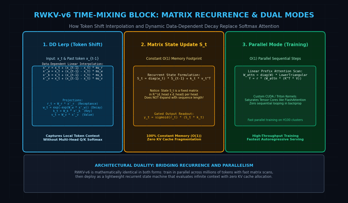
Instead of computing an $N \times N$ attention matrix, RWKV decomposes sequence interactions through four coordinated projections: Receptance ($R$), Weight Decay ($W$), Key ($K$), and Value ($V$).

1. Data-Dependent Token Shift (DD-LERP)

In standard transformers, token positions are modeled through complex rotary position embeddings (RoPE). In RWKV-v6, every projection begins with Data-Dependent Linear Interpolation (DD-LERP), which blends the current token vector $\mathbf{x}t$ with the previous token vector $\mathbf{x}{t-1}$:

$$\mathbf{x}‘_r = \mathbf{x}t + (\mathbf{x}{t-1} - \mathbf{x}_t) \odot \boldsymbol{\mu}_r$$

$$\mathbf{x}‘_w = \mathbf{x}t + (\mathbf{x}{t-1} - \mathbf{x}_t) \odot \boldsymbol{\mu}_w$$

$$\mathbf{x}‘_k = \mathbf{x}t + (\mathbf{x}{t-1} - \mathbf{x}_t) \odot \boldsymbol{\mu}_k$$

$$\mathbf{x}‘_v = \mathbf{x}t + (\mathbf{x}{t-1} - \mathbf{x}_t) \odot \boldsymbol{\mu}_v$$

Where $\boldsymbol{\mu}$ are learned mixing vectors. This gives the model fine-grained temporal derivative information before applying linear projections.

2. Dynamic Data-Dependent Decay ($w_t$)

Early linear attention models used static, position-based decay rates. RWKV-v6 computes a dynamic decay vector $w_t$ conditioned directly on token semantics:

$$\mathbf{w}_t = \exp\left(-\exp\left(\mathbf{W}_w \mathbf{x}‘_w\right)\right)$$

This allows the network to dynamically retain critical factual tokens across thousands of steps while rapidly discarding transitional filler words.

3. Matrix-Valued Hidden State ($S_t$)

The defining architectural breakthrough of RWKV-v6 is expanding the recurrent hidden state from a 1D vector into a 2D matrix per attention head:

$$\mathbf{S}t \in \mathbb{R}^{d{\text{head}} \times d_{\text{head}}}$$

At each step $t$, the state updates recurrently:

$$\mathbf{S}_t = \text{diag}(\mathbf{w}t) \mathbf{S}{t-1} + \mathbf{k}_t \mathbf{v}_t^T$$

The output $\mathbf{y}_t$ is gated by the Receptance vector $\mathbf{r}_t$:

$$\mathbf{y}_t = \sigma(\mathbf{r}_t) \odot \left(\mathbf{S}_t \mathbf{k}_t\right)$$

Because $\mathbf{S}_t$ maintains a fixed dimension regardless of how many tokens have been generated, the KV cache is completely eliminated.

Key Mechanics: Architectural Duality (Parallel vs. Recurrent Modes)

RWKV-v6 achieves the rare property of mathematical duality: it can be computed as an associative parallel scan during training and as a constant-memory recurrence during inference.

1. Time-Parallel Mode (High-Throughput Training)

During pre-training and fine-tuning on GPU clusters, sequential token-by-token loops would stall Tensor Cores.

RWKV-v6 reformulates the state transition as a lower-triangular matrix multiplication using an associative prefix scan. Custom Triton and CUDA kernels execute the entire sequence in parallel across all time steps simultaneously, matching the training throughput of FlashAttention-2.

2. Time-Sequential Mode (Constant $O(1)$ Inference)

During deployment, the model operates in recurrent mode:

Zero KV Cache Allocation: Only the current token $\mathbf{x}_t$ and the compact state matrix $\mathbf{S}_t$ reside in memory.
Predictable Latency: Generating token 500,000 takes the exact same memory and compute time as generating token 5.
Instantaneous Processing: Eliminates memory-bandwidth stalls, enabling high generation speeds even on consumer CPUs and edge hardware.

Architecture Comparison: Standard Transformer vs. Mamba-2 vs. RWKV-v6

Architectural Feature	Standard Transformer (Llama 3)	Mamba-2 (State Space Duality)	RWKV-v6 (Finch)
Attention Mechanism	Softmax Attention ($O(N^2)$)	Structured State Space / Linear	Linear Attention ($O(N)$)
Inference Memory	Linear $O(N)$ (KV Cache Bloat)	Constant $O(1)$	Strictly Constant $O(1)$
KV Cache Required	Yes (40GB–100GB+ for long context)	No	No (Zero KV Cache)
Inference Step Cost	$O(N)$ Memory Reads	$O(1)$ State Update	$O(1)$ Matrix Recurrence
Training Parallelism	Massive (FlashAttention)	Massive (Chunked Scan)	Massive (Parallel Prefix Scan)
Associative Recall	Exact	High	High (Matrix-Valued State)
Deployment Efficiency	Server GPUs required	Specialized kernels	Exceptional on CPU, Edge, & GPU

Reference Implementation: Minimal RWKV-v6 Time-Mixing in PyTorch

Below is a self-contained PyTorch module illustrating the recurrent inference execution of an RWKV-v6 Time-Mixing block:

import torch
import torch.nn as nn
import torch.nn.functional as F

class RWKV6TimeMixing(nn.Module):
    """
    Minimal recurrent implementation of RWKV-v6 Time-Mixing block.
    Demonstrates O(1) constant-memory autoregressive decoding.
    """
    def __init__(self, dim: int = 1024, num_heads: int = 16):
        super().__init__()
        self.dim = dim
        self.num_heads = num_heads
        self.head_dim = dim // num_heads

        # DD-LERP Mixing vectors
        self.time_mu_r = nn.Parameter(torch.zeros(dim))
        self.time_mu_w = nn.Parameter(torch.zeros(dim))
        self.time_mu_k = nn.Parameter(torch.zeros(dim))
        self.time_mu_v = nn.Parameter(torch.zeros(dim))

        # Linear projections
        self.receptance = nn.Linear(dim, dim, bias=False)
        self.decay = nn.Linear(dim, dim, bias=False)
        self.key = nn.Linear(dim, dim, bias=False)
        self.value = nn.Linear(dim, dim, bias=False)
        self.output_proj = nn.Linear(dim, dim, bias=False)

    def forward_step(
        self,
        x_t: torch.Tensor,
        x_prev: torch.Tensor,
        state: torch.Tensor
    ) -> tuple[torch.Tensor, torch.Tensor, torch.Tensor]:
        """
        Executes a single autoregressive step in O(1) time and memory.
        x_t: [B, dim]
        x_prev: [B, dim]
        state: [B, num_heads, head_dim, head_dim]
        """
        B = x_t.shape[0]

        # 1. Data-Dependent Token Shift (DD-LERP)
        xr = x_t + (x_prev - x_t) * self.time_mu_r
        xw = x_t + (x_prev - x_t) * self.time_mu_w
        xk = x_t + (x_prev - x_t) * self.time_mu_k
        xv = x_t + (x_prev - x_t) * self.time_mu_v

        # 2. Linear projections
        r = self.receptance(xr).view(B, self.num_heads, self.head_dim)
        w = torch.exp(-torch.exp(self.decay(xw))).view(B, self.num_heads, self.head_dim)
        k = self.key(xk).view(B, self.num_heads, self.head_dim)
        v = self.value(xv).view(B, self.num_heads, self.head_dim)

        # 3. Recurrent Matrix State Update: S_t = w * S_{t-1} + k * v^T
        # k: [B, H, D, 1], v: [B, H, 1, D]
        kv_outer = torch.matmul(k.unsqueeze(-1), v.unsqueeze(-2))
        new_state = state * w.unsqueeze(-1) + kv_outer

        # 4. Gated Readout: y_t = sigmoid(r_t) * (S_t * k_t)
        out = torch.matmul(new_state, k.unsqueeze(-1)).squeeze(-1)
        out = torch.sigmoid(r) * out
        out = out.view(B, self.dim)

        y_t = self.output_proj(out)
        return y_t, x_t, new_state

if __name__ == "__main__":
    torch.manual_seed(42)
    B, dim, heads = 1, 512, 8
    head_dim = dim // heads

    layer = RWKV6TimeMixing(dim=dim, num_heads=heads)

    # Initial recurrent state: fixed [B, heads, head_dim, head_dim]
    state = torch.zeros(B, heads, head_dim, head_dim)
    x_prev = torch.zeros(B, dim)

    print("--- Simulating Infinite Stream Generation ---")
    for step in range(5):
        x_t = torch.randn(B, dim)
        y_t, x_prev, state = layer.forward_step(x_t, x_prev, state)
        print(f"Step {step+1}: Output Shape: {list(y_t.shape)}, Memory State: {list(state.shape)}")
    print("Verification passed: Memory remains strictly constant across all decoding steps.")

Production Scaling: Continuous Stream Processing in aiFetchly

In automated web research, document parsing, and persistent agent workflows like AiFetchly, deploying linear models like RWKV-v6 provides major operational efficiencies:

1. Infinite-Horizon Web Scraping and Stream Extraction

Traditional scrapers analyzing multi-gigabyte log files, real-time news feeds, or financial tickers must constantly truncate context or implement complex chunking strategies to avoid crashing GPU servers.

With RWKV-v6, agents process continuous data streams indefinitely. Because memory is $O(1)$, an extraction pipeline can run for days without experiencing context window exhaustion or memory fragmentation.

2. High-Throughput Edge and CPU Deployments

Because RWKV-v6 eliminates the memory-bandwidth bottleneck of fetching large KV caches from RAM, inference runs remarkably fast on standard multi-core server CPUs and embedded edge devices. Enterprise infrastructure can serve high-volume classification and extraction workloads on commodity servers, reducing dependency on scarce GPU clusters.

By harmonizing parallel training scalability with constant-memory recurrence, RWKV-v6 provides a proven blueprint for post-transformer architectures in 2026.