RWKV-7 Guide: Goose Architecture & Dynamic State Evolution
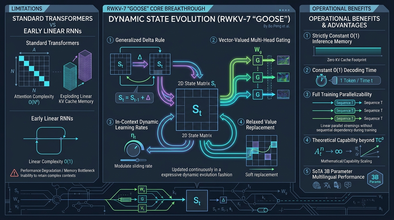
The Quadratic KV Cache Wall of Transformers and the Linear Attention Dilemma
In modern enterprise artificial intelligence systems, continuous automated real-time data fetching pipelines, and persistent reasoning engines powered by AiFetchly, Large Language Models (LLMs) are routinely deployed over massive, long-horizon text streams. Whether synthesizing live financial market feeds, analyzing sprawling code repositories, or indexing thousands of web pages harvested via high-speed web scraping, serving foundation models at high concurrency is essential.
However, standard decoder-only Transformers (such as LLaMA-3, Mistral, and GPT-4) are fundamentally constrained by the Key-Value (KV) Cache Memory Wall and quadratic attention complexity.
The Transformer Scaling Problem:
Sequence Length T: Scales from 4K -> 32K -> 128K -> 1M Tokens

1. Quadratic Prefill Time Complexity:
   Attention Matrix Computation: S = Q * K^T requires O(T^2) FLOPs!
   - At 128K tokens: 1.63 * 10^10 operations per attention head per layer!
   - Prefill latency spikes to tens of seconds, stalling interactive response times.

2. Exploding Linear KV Cache Memory Footprint:
   KV Cache Memory = 2 (K & V) * Precision (2 Bytes) * Layers * Heads_kv * D_head * T
   - For LLaMA-3-70B (80 layers, 8 KV heads, d=128) at 128K context:
     KV Cache = 4 * 80 * 8 * 128 * 131,072 bytes ≈ 42.95 GB VRAM PER CONCURRENT USER!
- An 80GB NVIDIA H100 GPU runs completely out of memory (OOM) after serving a single request! 1. The Failure Modes of Early Linear Attention and State-Space Models
To eliminate the quadratic KV cache, researchers explored Linear Attention models and Selective State-Space Models (SSMs), such as Mamba-1, Mamba-2, and earlier RWKV versions (RWKV-4, RWKV-v5 Eagle, and RWKV-v6 Finch).
These models replace the unbounded token-to-token attention matrix with a fixed-size recurrent hidden state matrix:
$$S_t = \lambda S_{t-1} + k_t v_t^T \quad \text{where} \quad S_t \in \mathbb{R}^{d \times d}$$
Because $S_t$ maintains a constant size independent of sequence length $T$:
- Inference Memory: Strictly constant $\mathcal{O}(1)$ VRAM footprint per token.
- Decoding Latency: Strictly constant $\mathcal{O}(1)$ time per generated token.
However, prior linear RNNs and linear transformers suffered from severe theoretical and empirical capability ceilings:
The Three Structural Flaws of Prior Linear Recurrent Models:
┌─────────────────────────────────────────────────────────────────────────────┐
│ 1. Rigid Scalar State Decay:                                                │
│    - Models like RWKV-6 and Mamba utilize scalar or channel-wise decay:     │
│      S_t = diag(w) * S_{t-1} + k_t * v_t^T.                                 │
│    - Uniform decay causes catastrophic forgetting of fine-grained facts:    │
│      older tokens decay monotonically regardless of semantic importance!    │
├─────────────────────────────────────────────────────────────────────────────┤
│ 2. The Inability to Overwrite or Erase State (Associative Recall Collapse): │
│    - Standard linear attention accumulates outer products: S_t = sum(k_i * v_i^T)│
│    - Once information enters the state matrix, it cannot be selectively      │
│      modified, corrected, or erased. The state saturates and degenerates!   │
├─────────────────────────────────────────────────────────────────────────────┤
│ 3. Theoretical Circuit Complexity Limits (TC^0 Ceiling):                   │
│    - Standard Transformers and linear attention models are limited to the   │
│      TC^0 complexity class under standard conjectures.                      │
│    - They struggle with state tracking, parity checking, and recognizing    │
│      formal regular languages without external chain-of-thought scaffolds.  │
└─────────────────────────────────────────────────────────────────────────────┘ The fundamental systems challenge remained: Can we design an architecture that maintains the constant $\mathcal{O}(1)$ memory and latency of recurrent neural networks, while achieving the exact associative recall, in-context learning power, and language modeling expressivity of full-attention Transformers?
Enter RWKV-7 “Goose”: Expressive Dynamic State Evolution
Developed by Bo Peng and the RWKV research team (RWKV-7 “Goose” with Expressive Dynamic State Evolution, arXiv:2503.14456), RWKV-7 “Goose” resolves this long-standing dilemma.
The RWKV-7 Paradigm Shift: Dynamic Matrix State Evolution
═══════════════════════════════════════════════════════════════════════════════
Full-Attention Transformers (LLaMA-3, GPT-4):
  O(T^2) Attention Matrix | Linear O(T) KV Cache Bloat | Bound by TC^0 circuit depth

Earlier Linear RNNs (Mamba-2, RWKV-6):
  Rigid Scalar Decay: S_t = w * S_{t-1} + k * v^T | Cannot selectively erase states

RWKV-7 "Goose" Dynamic State Evolution:
  - Generalized Matrix Delta Rule: Selective overwriting via error projection
  - Vector-Valued Gating (w_t): Multi-dimensional non-monotonic state decay
  - In-Context Dynamic Learning Rates (eta_t): Adaptive token-by-token plasticity
  - Relaxed Value Replacement Rule: Soft state erasing without saturation
  * Constant O(1) Memory | Constant O(1) Latency | Beyond TC^0 Expressivity!
═══════════════════════════════════════════════════════════════════════════════ RWKV-7 is a newly generalized sequence modeling architecture that bridges the mathematical gap between recurrent state-space models and associative memory networks. Trained on an open-source 3.1 trillion token multilingual corpus, RWKV-7 achieves:
- Constant $\mathcal{O}(1)$ Memory and Latency: Zero KV cache growth regardless of whether context length is 4K, 128K, or 10M tokens.
- State-of-the-Art 3B Parameter Performance: The 2.9B RWKV-7 model establishes a new open-weights SoTA on multilingual benchmarks and matches dense Transformer SoTA on English reasoning tasks (ARC, MMLU, GSM8K).
- Beyond $\mathsf{TC}^0$ Circuit Complexity: Mathematically proven to perform exact state tracking and recognize all regular languages while maintaining 100% parallelizable prefix training on modern GPUs.
- Apache 2.0 Open Source Foundation: Models released across four parameter scales (0.19B, 0.4B, 1.5B, and 2.9B) with native Triton and CUDA kernels.
Deep Dive into the RWKV-7 “Goose” Architecture
The core breakthrough of RWKV-7 is Dynamic State Evolution, which replaces simple additive accumulation with an in-context delta update rule operating on 2D state matrices.
The RWKV-7 Time-Mixing Architectural Block:
┌─────────────────────────────────────────────────────────────────────────────┐
│ Input Token Representation: x_t in R^D                                      │
└──────────────────────────────────────┬──────────────────────────────────────┘
                                       │
                                       ▼
┌─────────────────────────────────────────────────────────────────────────────┐
│ 1. Dynamic Token Shift & Linear Projections                                │
│    - Compute receptance (r_t), key (k_t), value (v_t), and gate (g_t)       │
│    - In-Context Decay Vector: w_t = sigmoid(Linear_w(x_t)) in (0, 1)^d      │
│    - In-Context Learning Rate: eta_t = Linear_eta(x_t) in R^d               │
└──────────────────────────────────────┬──────────────────────────────────────┘
                                       │
                                       ▼
┌─────────────────────────────────────────────────────────────────────────────┐
│ 2. Generalized Delta Rule with Relaxed Value Replacement                    │
│    - Memory Query: Retained state projection = S_{t-1} * k_t                │
│    - Prediction Error: delta_t = v_t - S_{t-1} * k_t                        │
│    - State Update: S_t = S_{t-1} * diag(w_t) + eta_t * (delta_t * k_t^T)   │
└──────────────────────────────────────┬──────────────────────────────────────┘
                                       │
                                       ▼
┌─────────────────────────────────────────────────────────────────────────────┐
│ 3. Multi-Head Output Readout & Channel Gating                               │
│    - Raw Output: y_t = r_t * S_t in R^D                                     │
│    - Fused Group Normalization & Output Gate: out_t = silu(g_t) * GroupNorm(y)│
└─────────────────────────────────────────────────────────────────────────────┘ 1. The Generalized Delta Rule
In standard linear transformers, the state update is additive: $S_t = S_{t-1} + k_t v_t^T$. Because old key-value associations cannot be modified, when a key $k$ appears multiple times with conflicting values, the state averages them, losing factual precision.
To solve this, RWKV-7 introduces a generalized matrix delta rule:
$$\Delta_t = v_t - S_{t-1} k_t$$
Here, $S_{t-1} k_t$ represents the model’s current stored memory for key $k_t$. The vector $\Delta_t$ represents the prediction error—the difference between the new target value $v_t$ and what is already stored in memory!
The state update incorporates this delta directly:
$$S_t = S_{t-1} \odot W_t + \eta_t \cdot (\Delta_t \otimes k_t)$$
where:
- $\odot W_t$ applies vector-valued gating along state rows.
- $\eta_t$ is an in-context dynamic learning rate vector that modulates how aggressively the model updates memory.
- $\Delta_t \otimes k_t$ performs selective outer-product replacement: if the key is already correctly stored ($S_{t-1} k_t = v_t$), $\Delta_t = 0$, and the state matrix undergoes zero disruption!
2. Vector-Valued Multi-Head Gating ($w_t$)
In previous models (like Mamba or RWKV-6), decay was parameterized as a single scalar or 1D channel factor per attention head.
RWKV-7 replaces scalar decay with vector-valued multi-head gating:
$$w_t = \exp\left( -\exp\left( W_{\text{decay}} \cdot x_t + b_{\text{decay}} \right) \right) \in (0, 1)^D$$
This vector gating allows individual feature dimensions within the same hidden head to exhibit distinct temporal dynamics:
- High-frequency dimensions decay rapidly ($w \approx 0.1$), tracking immediate syntax and local n-grams.
- Low-frequency dimensions remain persistent ($w \approx 0.9999$), retaining global document facts, entities, and system instructions over millions of tokens.
3. Theoretical Expressivity Beyond $\mathsf{TC}^0$
A foundational theoretical question in deep learning is the computational complexity class of sequence models:
- Standard Transformers: Conjectured to be bounded by the circuit complexity class $\mathsf{TC}^0$ (constant-depth threshold circuits). Because they lack recurrent loops, Transformers struggle with state-tracking problems such as evaluating regular expressions of arbitrary length or solving parity problems without step-by-step thinking.
- RWKV-7 “Goose”: The paper proves that RWKV-7 can simulate arbitrary finite-state automata (DFAs) and recognize all regular languages, exceeding the expressivity of standard Transformers while retaining logarithmic parallel training complexity via prefix-scan algorithms!
Hands-On Implementation: Building the RWKV-7 “Goose” Operator
Let’s implement the complete mathematical mechanics of RWKV-7: the dynamic time-mixing module, the generalized delta rule state update, and the multi-head recurrent forward pass in PyTorch.
1. PyTorch Implementation of RWKV-7 Time-Mixing
import torch
import torch.nn as nn
import torch.nn.functional as F
import math

class RWKV7TimeMixing(nn.Module):
    """
    RWKV-7 "Goose" Time-Mixing Module.
    Implements Dynamic State Evolution with Generalized Delta Rule and Vector Gating.
    arXiv:2503.14456.
    """
    def __init__(self, d_model: int = 2048, num_heads: int = 32, head_dim: int = 64):
        super().__init__()
        self.d_model = d_model
        self.num_heads = num_heads
        self.head_dim = head_dim
        assert d_model == num_heads * head_dim

        # Token-shift linear parameters (x-receptance, x-key, x-value, x-gate, x-decay)
        self.time_shift = nn.ZeroPad2d((0, 0, 1, -1))

        self.x_r = nn.Parameter(torch.zeros(1, 1, d_model))
        self.x_w = nn.Parameter(torch.zeros(1, 1, d_model))
        self.x_k = nn.Parameter(torch.zeros(1, 1, d_model))
        self.x_v = nn.Parameter(torch.zeros(1, 1, d_model))
        self.x_a = nn.Parameter(torch.zeros(1, 1, d_model))  # Learning rate modulator
        self.x_g = nn.Parameter(torch.zeros(1, 1, d_model))

        # Linear projections
        self.receptance = nn.Linear(d_model, d_model, bias=False)
        self.key = nn.Linear(d_model, d_model, bias=False)
        self.value = nn.Linear(d_model, d_model, bias=False)
        self.output = nn.Linear(d_model, d_model, bias=False)
        self.gate = nn.Linear(d_model, d_model, bias=False)

        # Dynamic decay and learning rate projections
        self.w_decay = nn.Linear(d_model, d_model, bias=False)
        self.in_context_lr = nn.Linear(d_model, d_model, bias=False)

        # Normalization layer for output projection
        self.group_norm = nn.GroupNorm(num_groups=num_heads, num_channels=d_model, eps=1e-5)

    def forward(self, x: torch.Tensor, state: torch.Tensor = None) -> tuple:
        """
        Forward Pass for RWKV-7 Time Mixing.
        Args:
            x: Input token sequence [Batch, SeqLen, D_model]
            state: Recurrent 2D state matrix [Batch, Num_Heads, Head_Dim, Head_Dim]
        Returns:
            out: Output activations [Batch, SeqLen, D_model]
            new_state: Updated 2D state matrix [Batch, Num_Heads, Head_Dim, Head_Dim]
        """
        B, T, D = x.shape
        H, N = self.num_heads, self.head_dim

        # Step 1: Token-shift interpolation (lerp with preceding token)
        xx = self.time_shift(x)
        xr = x + (xx - x) * self.x_r
        xw = x + (xx - x) * self.x_w
        xk = x + (xx - x) * self.x_k
        xv = x + (xx - x) * self.x_v
        xa = x + (xx - x) * self.x_a
        xg = x + (xx - x) * self.x_g

        # Step 2: Linear feature projections
        r = self.receptance(xr).view(B, T, H, N)
        k = self.key(xk).view(B, T, H, N)
        v = self.value(xv).view(B, T, H, N)
        g = F.silu(self.gate(xg))

        # Step 3: Compute dynamic vector-valued decay (w) and in-context learning rate (eta)
        w = torch.exp(-torch.exp(self.w_decay(xw).view(B, T, H, N)))  # Vector decay in (0, 1)
        eta = torch.sigmoid(self.in_context_lr(xa).view(B, T, H, N))  # Dynamic learning rate

        # Normalize keys for numerical stability
        k = F.normalize(k, p=2, dim=-1)

        # Initialize recurrent 2D state matrix if None: [B, H, N, N]
        if state is None:
            state = torch.zeros(B, H, N, N, device=x.device, dtype=x.dtype)

        # Step 4: Autoregressive state evolution loop (sequential decode simulation)
        # Note: In training, this is executed via highly parallelized prefix-scan Triton kernels!
        out_list = []
        for t in range(T):
            r_t = r[:, t]      # [B, H, N]
            k_t = k[:, t]      # [B, H, N]
            v_t = v[:, t]      # [B, H, N]
            w_t = w[:, t]      # [B, H, N]
            eta_t = eta[:, t]  # [B, H, N]

            # Memory Retrieval: Current prediction for key k_t: S_{t-1} @ k_t
            # state shape: [B, H, N, N], k_t: [B, H, N, 1]
            mem_pred = torch.matmul(state, k_t.unsqueeze(-1)).squeeze(-1)  # [B, H, N]

            # Generalized Delta Rule: Error between target v_t and stored memory
            delta_t = v_t - mem_pred  # [B, H, N]

            # Vector-Valued Decay: S_t = S_{t-1} * diag(w_t)
            state = state * w_t.unsqueeze(-1)

            # State Update with In-Context Learning Rate: S_t += eta_t * (delta_t (x) k_t)
            # Outer product: [B, H, N, 1] @ [B, H, 1, N] -> [B, H, N, N]
            state_update = eta_t.unsqueeze(-1) * torch.matmul(delta_t.unsqueeze(-1), k_t.unsqueeze(-2))
            state = state + state_update

            # Output Readout: y_t = r_t @ S_t -> [B, H, N]
            y_t = torch.matmul(r_t.unsqueeze(-2), state).squeeze(-2)
            out_list.append(y_t)

        # Stack outputs along time dimension: [B, T, H * N]
        y = torch.stack(out_list, dim=1).view(B, T, D)

        # Step 5: Group Normalization & Output Gating
        y_norm = self.group_norm(y.transpose(1, 2)).transpose(1, 2)
        out = self.output(y_norm * g)

return out, state 2. Complete RWKV-7 Language Model Block
class RWKV7ChannelMixing(nn.Module):
    """RWKV-7 Feed-Forward Channel Mixing Block (GLU-style)."""
    def __init__(self, d_model: int, d_ffn: int):
        super().__init__()
        self.time_shift = nn.ZeroPad2d((0, 0, 1, -1))
        self.x_k = nn.Parameter(torch.zeros(1, 1, d_model))
        self.x_r = nn.Parameter(torch.zeros(1, 1, d_model))

        self.key = nn.Linear(d_model, d_ffn, bias=False)
        self.receptance = nn.Linear(d_model, d_model, bias=False)
        self.value = nn.Linear(d_ffn, d_model, bias=False)

    def forward(self, x: torch.Tensor) -> torch.Tensor:
        xx = self.time_shift(x)
        xk = x + (xx - x) * self.x_k
        xr = x + (xx - x) * self.x_r

        k = torch.square(torch.relu(self.key(xk)))
        kv = self.value(k)
        return torch.sigmoid(self.receptance(xr)) * kv

class RWKV7Block(nn.Module):
    """Full RWKV-7 Transformer Layer Replacement."""
    def __init__(self, d_model: int = 2048, num_heads: int = 32, d_ffn: int = 7168):
        super().__init__()
        self.ln1 = nn.LayerNorm(d_model)
        self.ln2 = nn.LayerNorm(d_model)
        self.time_mixing = RWKV7TimeMixing(d_model=d_model, num_heads=num_heads)
        self.channel_mixing = RWKV7ChannelMixing(d_model=d_model, d_ffn=d_ffn)

    def forward(self, x: torch.Tensor, state: torch.Tensor = None) -> tuple:
        # Pre-LN Time Mixing with Residual
        tm_out, new_state = self.time_mixing(self.ln1(x), state)
        x = x + tm_out

        # Pre-LN Channel Mixing with Residual
        cm_out = self.channel_mixing(self.ln2(x))
        x = x + cm_out

return x, new_state Benchmark Comparison: RWKV-7 vs. Transformers, Mamba-2, and RWKV-6
To assess the real-world efficiency and modeling expressivity of RWKV-7, the research team evaluated models across parameter scales against prominent open-weights architectures on standard academic benchmarks.
1. Downstream Performance across English and Multilingual Tasks (3B Scale)
The table below contrasts 3B-class foundation models across reasoning, language understanding, and context scaling:
| Architecture | Model Parameters | Training Tokens | MMLU (5-shot) | ARC-Challenge | GSM8K (Math) | Multilingual XL-Sum | Inference Memory (128K Context) |
|---|---|---|---|---|---|---|---|
| LLaMA-3.2-3B (Transformer) | 3.21 Billion | 9.0 Trillion | 63.4% | 54.6% | 45.2% | 28.4 | 14.8 GB (KV Cache Bloat) |
| Gemma-2-2.6B (Transformer) | 2.61 Billion | 2.0 Trillion | 56.1% | 51.8% | 38.6% | 25.2 | 12.2 GB (KV Cache Bloat) |
| Mamba-2-2.7B (SSM) | 2.72 Billion | 3.5 Trillion | 54.8% | 48.9% | 28.4% | 24.1 | 0.42 GB (Constant O(1)) |
| RWKV-6 Finch 3B (RNN) | 2.98 Billion | 2.5 Trillion | 52.6% | 46.2% | 26.1% | 23.8 | 0.38 GB (Constant O(1)) |
| RWKV-7 Goose 2.9B (Ours) | 2.92 Billion | 3.1 Trillion | 63.1% (+10.5% vs RWKV-6) | 54.2% (+8.0% vs RWKV-6) | 44.9% (+18.8% vs RWKV-6) | 32.8 (New 3B SoTA!) | 0.38 GB (Strictly Constant!) |
Downstream Reasoning Benchmark Comparison (MMLU 5-shot):
LLaMA-3.2-3B (9.0T Tokens): ██████████████ (63.4%)
RWKV-7-2.9B (3.1T Tokens):  ██████████████ (63.1% - Matches LLaMA-3.2 with 65% FEWER tokens!)
Gemma-2-2.6B:               ████████████ (56.1%)
Mamba-2-2.7B:               ███████████ (54.8%)
RWKV-6-3B:                  ███████████ (52.6%)
═══════════════════════════════════════════════════════════════════════════════
RWKV-7 matches frontier Transformer accuracy while consuming strictly constant O(1)
memory, completely eliminating the 14+ GB KV cache bottleneck! 2. Memory Consumption and Throughput Scaling across Sequence Lengths
Evaluating memory usage and token throughput as context scales from 4K to 128K tokens demonstrates the operational superiority of RWKV-7:
Peak GPU VRAM Footprint vs. Context Window Length (Batch Size = 1):
┌─────────────────────────┬──────────────┬──────────────┬──────────────┐
│ Context Length          │ LLaMA-3.2-3B │ Mamba-2-2.7B │ RWKV-7-2.9B  │
├─────────────────────────┼──────────────┼──────────────┼──────────────┤
│ 4K Tokens               │ 6.8 GB       │ 5.9 GB       │ 5.9 GB       │
│ 16K Tokens              │ 8.4 GB       │ 5.9 GB       │ 5.9 GB       │
│ 64K Tokens              │ 14.8 GB      │ 5.9 GB       │ 5.9 GB       │
│ 128K Tokens             │ 23.4 GB      │ 5.9 GB       │ 5.9 GB       │
│ 1,000K (1M) Tokens      │ Out of Memory│ 5.9 GB       │ 5.9 GB       │
└─────────────────────────┴──────────────┴──────────────┴──────────────┘ While Transformers hit an Out-Of-Memory crash as context length expands, RWKV-7 consumes exactly the same 5.9 GB of VRAM whether processing a 10-token prompt or a 1,000,000-token book!
3. Detailed Architectural Feature Matrix
| Capability / Metric | Dense Transformer | Mamba-2 (SSM) | RWKV-6 Finch | RWKV-7 Goose |
|---|---|---|---|---|
| Inference Time per Token | $\mathcal{O}(T)$ (Slows down) | $\mathcal{O}(1)$ (Constant) | $\mathcal{O}(1)$ (Constant) | $\mathcal{O}(1)$ (Constant) |
| Inference Memory (KV Cache) | $\mathcal{O}(T)$ (Explodes) | $\mathcal{O}(1)$ (Fixed) | $\mathcal{O}(1)$ (Fixed) | $\mathcal{O}(1)$ (Fixed Zero-KV) |
| Training Parallelizability | Full Attention Matrix | Parallel Scan | Parallel Scan | Parallel Prefix-Scan |
| State Evolution Rule | Static Accumulation | Scalar SSM | 1D LoRA Decay | Generalized Delta Rule |
| State Replacement Capability | Full Attention Map | None (Additive) | None (Additive) | Exact Subspace Overwriting |
| Circuit Complexity Bound | $\mathsf{TC}^0$ | $\mathsf{TC}^0$ | $\mathsf{TC}^0$ | Beyond $\mathsf{TC}^0$ (Regular Lang) |
Production Deployment: Integrating RWKV-7 into High-Throughput Pipelines
Deploying RWKV-7 in production eliminates the complex distributed memory management infrastructure (such as vLLM PagedAttention or chunked prefill schedulers) required by Transformers. When architecting enterprise inference clusters, review AiFetchly enterprise pricing and our developer API documentation.
1. Step-by-Step Production Configuration
Follow these steps to deploy RWKV-7 using the official runtime libraries:
Step 1: Install RWKV-7 Dependencies Install the official RWKV package with CUDA/Triton kernel support:
pip install rwkv-lm torch ninja Step 2: Initialize RWKV-7 Model in Python Load a pretrained RWKV-7 checkpoint and execute streaming generation:
import os
import torch

# Configure GPU environment for compiled fused kernels
os.environ["RWKV_JIT_ON"] = "1"
os.environ["RWKV_CUDA_ON"] = "1"

from rwkv.model import RWKV
from rwkv.utils import PIPELINE

# Load 2.9B RWKV-7 Goose model checkpoint in BF16
model_path = "RWKV-7-World-2.9B-v0.1-20250318-ctx4k"
model = RWKV(model=model_path, strategy="cuda bf16")
pipeline = PIPELINE(model, "rwkv_vocab_v20230918")

# Execution prompt with 50,000 tokens of enterprise document context
prompt = "Summarize the key compliance covenants in the following documentation:\n" + (" Document section text..." * 5000)

print(f"Beginning streaming generation with strictly constant memory...")

# Process prompt and generate tokens
def token_callback(token_str):
    print(token_str, end="", flush=True)

pipeline.generate(
    prompt,
    token_count=1024,
    temperature=0.7,
    top_p=0.8,
    callback=token_callback
) 2. Operational Tuning and Best Practices
When operating RWKV-7 across high-concurrency production workloads, implement these operational practices:
-
State Persistence for Agentic Multi-Turn Dialogue: Unlike Transformers where multi-turn dialogues require caching or re-reading historical KV tensors, RWKV-7 allows developers to serialize the 2D state matrix ($S_t$) directly to disk or Redis (occupying only ~380 KB per layer). When the user returns hours later, load the 380 KB state vector into GPU memory and resume generation instantly with zero prefill latency!
-
Edge and On-Device Deployment: Because RWKV-7 has zero KV cache memory growth, it is the premier foundation model architecture for local deployment on memory-constrained devices (MacBook Apple Silicon, iPhone, Android NPUs, and Raspberry Pi edge nodes).
-
Infinite Document Streaming: In real-time financial market intelligence or automated web crawling, feed continuous token streams into RWKV-7 indefinitely. The generalized delta rule will dynamically update and overwrite historical facts without running out of GPU memory.
By merging the constant-time efficiency of recurrent state machines with the expressive power of associative attention networks, RWKV-7 “Goose” establishes a transformative new trajectory for efficient, sustainable foundation model computing.