RetNet Guide: Retentive Networks & The Impossible Triangle
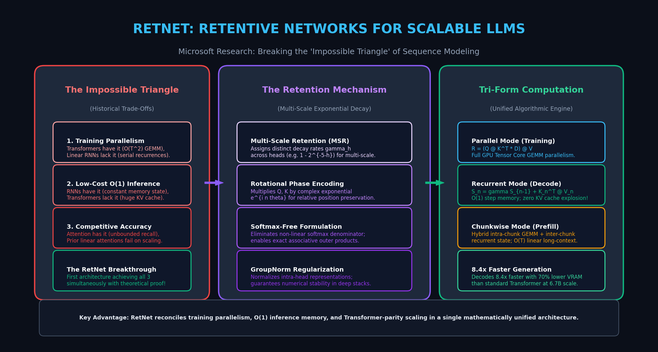
The Problem: The Impossible Triangle of Sequence Modeling
Since the advent of deep learning for natural language processing, sequential architectures have been constrained by an architectural trade-off known as “The Impossible Triangle” of sequence modeling.
For an architecture to serve as a universal foundation model backbone—powering high-throughput data extraction platforms, enterprise search pipelines, and autonomous desktop agents like AiFetchly—it must ideally possess three fundamental properties simultaneously:
- Training Parallelism: The ability to execute full sequence training in parallel across GPU Tensor Cores via dense matrix multiplications (GEMMs).
- Low-Cost Inference: Bounded $\mathcal{O}(1)$ step memory and constant-time token generation without an expanding state buffer.
- Competitive Performance: Uncompromised language modeling perplexity, in-context copying, and multi-hop reasoning on par with standard attention.
                  The Impossible Triangle

                  [Training Parallelism]
                          /\
                         /  \
                        /    \
                       /      \
      (Transformers)  /        \  (Linear Attention / RetNet)
                     /          \
                    /____________\
      [Low-Cost Inference]      [Competitive Performance]
(Recurrent RNNs) Historically, every major neural architecture could only satisfy two out of the three vertices:
1. Training Parallelism: The Transformer Moat
Standard Transformers achieve unmatched training parallelism and competitive performance through Multi-Head Self-Attention (MHA). Because self-attention computes all pairwise token interactions simultaneously ($Q K^T$), it parallelizes across the entire context length, maximizing GPU hardware saturation.
However, Transformers completely sacrifice low-cost inference:
- The Linear KV Cache Expansion: During autoregressive decoding, the Key-Value (KV) cache grows linearly $\mathcal{O}(T)$ with sequence length. Caching 128,000 tokens for an 8B model requires over 16 GB of GPU High-Bandwidth Memory (HBM) solely for historical activations.
- Memory Bandwidth Bottleneck: Decoding single tokens requires streaming tens of gigabytes of cached keys and values across the memory bus, keeping Tensor Cores idle and capping serving concurrency.
2. Low-Cost Inference: The Linear Attention and RNN Promise
Recurrent Neural Networks (RNNs) and early Linear Attention models (such as Katharopoulos et al.) achieve low-cost inference by compressing sequence history into a fixed-size recurrent state vector:
$$s_t = s_{t-1} + \phi(k_t) v_t^T, \quad o_t = \phi(q_t) s_t$$
During generation, memory consumption is strictly $\mathcal{O}(1)$ constant, and inference time is $\mathcal{O}(1)$ per token.
However, historical linear attention models failed on competitive performance:
- Removing the non-linear softmax operator causes the recurrent state to degrade into a noisy, unbounded sum, destroying associative recall, syntax preservation, and in-context learning.
- Furthermore, classic RNNs lack training parallelism, forcing sequential recurrent execution that cannot saturate modern AI accelerators.
3. Good Performance: The In-Context Associative Recall Wall
State Space Models (like Mamba-1) and gated linear RNNs introduced selective parameters to improve expressivity. While effective, pure 1D state vectors still encounter performance degradation on long-range needle-in-a-haystack retrieval and complex multi-hop extraction compared to standard Transformers.
The deep learning community widely believed that the impossible triangle was mathematically immutable. RetNet proves that the triangle can be broken.
The Core Architecture: The Retention Mechanism
Introduced by Microsoft Research and Tsinghua University (Sun et al., 2023), RetNet (Retentive Network) replaces Multi-Head Attention with a novel dual-form mathematical operator: Multi-Scale Retention (MSR).
Retention achieves Transformer-equivalent performance while natively admitting three mathematically equivalent computational paradigms: parallel, recurrent, and chunkwise recurrent.
1. Mathematical Formulation: From Softmax Attention to Retention
In standard self-attention, token representations are mixed via normalized exponential dot-products:
$$\text{Attention}(Q, K, V) = \text{softmax}\left(\frac{Q K^T}{\sqrt{d}}\right) V$$
The softmax function couples all tokens dynamically, which makes step-by-step recurrent formulation without caching historical keys mathematically impossible.
Retention discards the non-linear softmax denominator and instead injects explicit exponential temporal decay combined with complex rotational position embeddings.
Given an input sequence $X \in \mathbb{R}^{T \times d}$, Retention computes projections:
$$Q = X W_Q, \quad K = X W_K, \quad V = X W_V$$
Where $W_Q, W_K, W_V \in \mathbb{R}^{d \times d}$.
2. Relative Position via Complex Exponential Phase Rotations
Rather than injecting additive positional encodings, Retention applies a continuous complex rotational transformation to Query and Key vectors:
$$q_n = (X_n W_Q) e^{i n \theta}, \quad k_n = (X_n W_K) e^{-i n \theta}$$
Where $\theta \in \mathbb{R}^d$ is a learnable spatial frequency vector. When computing the inner product between query $q_n$ and key $k_m$:
$$q_n k_m^T = (X_n W_Q) e^{i(n - m)\theta} (X_m W_K)^T$$
The phase difference depends strictly on the relative distance $(n - m)$, providing an innate, continuous relative positional bias.
3. Multi-Scale Retention (MSR): Hierarchical Temporal Decay
To prevent unbounded activation growth in the absence of softmax normalization, Retention modulates token interactions using an explicit scalar decay factor $\gamma \in (0, 1)$.
In a Multi-Scale Retention (MSR) module with $H$ retention heads, each head is assigned a distinct, fixed decay parameter $\gamma$:
$$\gamma = 1 - 2^{-5 - h}, \quad \text{for head } h \in {1, \dots, H}$$
- Heads with large $\gamma$ (e.g., $\gamma = 0.996$): Experience very slow temporal decay, allowing them to capture long-range semantic dependencies and global document context.
- Heads with small $\gamma$ (e.g., $\gamma = 0.850$): Experience rapid temporal decay, forcing them to focus on immediate adjacent tokens, local syntactic rules, and grammatical parsing.
The Tri-Form Representations: One Formula, Three Modes
The defining innovation of RetNet is that the exact same mathematical formulation can be executed in three distinct computational modes depending on the operational requirement.
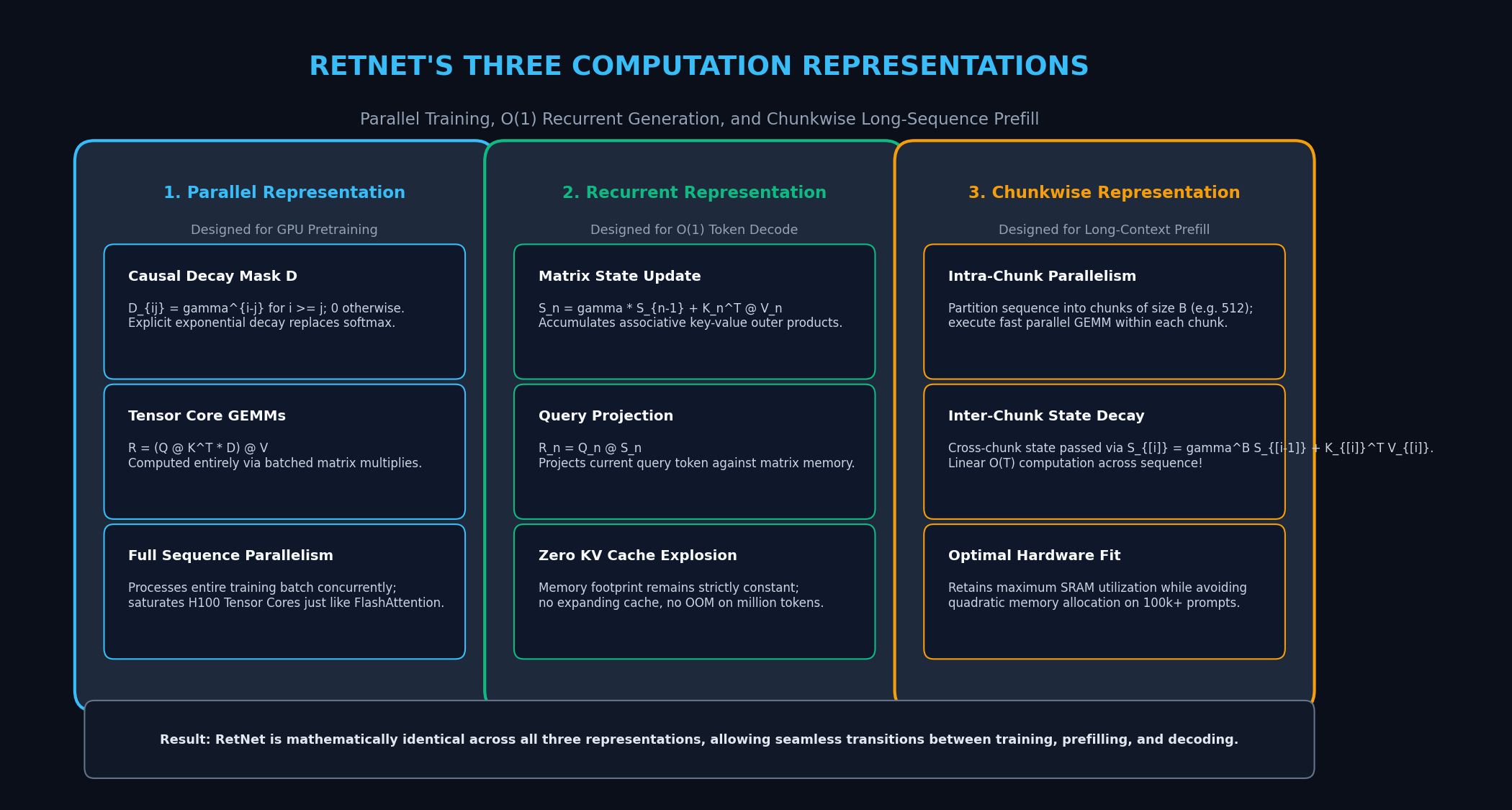
1. The Parallel Representation for High-Throughput Pretraining
During offline pretraining on massive web corpora, sequence lengths are fixed (e.g., 2,048 or 4,096 tokens). RetNet evaluates all tokens in parallel using standard matrix multiplications.
We construct a causal decay matrix $D \in \mathbb{R}^{T \times T}$ whose entries are defined by:
$$D_{ij} = \begin{cases} \gamma^{i - j} & \text{if } i \ge j \ 0 & \text{if } i < j \end{cases}$$
The parallel Retention output is computed as:
$$R = \left( (Q K^T) \odot D \right) V$$
$$\text{MSR}(X) = \text{GroupNorm}\left(\text{Concat}(R_1, \dots, R_H)\right) W_O$$
Because $Q K^T$ and $(Q K^T \odot D) V$ are standard matrix multiplications, they execute at maximum arithmetic intensity on GPU Tensor Cores, fully saturating NVIDIA H100 and B200 hardware.
2. The Recurrent Representation for Constant-Memory O(1) Decoding
During autoregressive token generation, computing attention against an expanding sequence history is wasteful. RetNet rewrites the retention operator as a linear recurrence:
$$S_n = \gamma S_{n-1} + K_n^T V_n \in \mathbb{R}^{d \times d}$$
$$R_n = Q_n S_n \in \mathbb{R}^{1 \times d}$$
Operational Mechanics:
- The recurrent state $S_n$ is a $d \times d$ matrix that acts as an associative memory store, accumulating key-value outer products weighted by exponential decay factor $\gamma$.
- To emit token $n$, the query vector $Q_n$ simply multiplies the existing state matrix $S_n$.
- The memory footprint is strictly $\mathcal{O}(1)$ constant. Generating token 100,000 consumes the exact same memory and latency as generating token 1!
3. The Chunkwise Recurrent Representation for Ultra-Long Sequence Prefill
When processing massive long-context documents (e.g., 100,000+ tokens) during prompt ingestion, pure parallel mode requires $\mathcal{O}(T^2)$ memory, while pure recurrent mode is slow on GPUs.
RetNet resolves this by introducing the Chunkwise Recurrent Representation:
- The sequence of length $T$ is divided into $N$ non-overlapping chunks of length $B$ (e.g., $B = 512$ tokens): $X = [X_{[1]}, X_{[2]}, \dots, X_{[N]}]$.
- Intra-Chunk Parallelism: Inside each chunk $i$, representations are computed in parallel using high-speed Tensor Core GEMMs.
- Inter-Chunk Recurrence: Between chunks, a recurrent state $S_{[i]}$ is passed forward, decayed by $\gamma^B$:
$$S_{[i]} = \gamma^B S_{[i-1]} + K_{[i]}^T V_{[i]} \in \mathbb{R}^{d \times d}$$
$$R_{[i]} = ((Q_{[i]} K_{[i]}^T) \odot D) V_{[i]} + (Q_{[i]} S_{[i-1]}) \odot \zeta$$
Where $\zeta_{j} = \gamma^{j+1}$ scales the influence of the historical cross-chunk state.
Chunkwise recurrence achieves linear $\mathcal{O}(T)$ compute complexity and constant memory during prompt prefill, enabling single-GPU processing of massive document contexts.
4. Comparison Table: Sequence Modeling Architectures
| Dimension | Standard Transformer (MHA) | Linear Attention (Katharopoulos) | Mamba-2 (SSD) | RetNet (Multi-Scale Retention) |
|---|---|---|---|---|
| Non-Linearity | Softmax on attention matrix | Kernel trick $\phi(x)$ | Input-dependent selective $\Delta$ | Exponential decay mask $D$ |
| Positional Encoding | RoPE / ALiBi / Absolute | Difficult to inject | Implicit in SSM discretization | Complex Exponential Rotation ($e^{in\theta}$) |
| Training Speed | Fast ($\mathcal{O}(T^2)$ GEMM) | Fast ($\mathcal{O}(T)$ Linear) | Fast (Chunked GEMM) | Fast ($\mathcal{O}(T^2)$ / $\mathcal{O}(T)$ Chunked) |
| Inference Step Memory | $\mathcal{O}(T)$ Expanding KV Cache | $\mathcal{O}(1)$ Constant | $\mathcal{O}(1)$ Constant | $\mathcal{O}(1)$ Constant Matrix State |
| Multi-Scale Gating | Implicit in attention heads | None (uniform sum) | Gated scalar states | Explicit Decay $\gamma_h$ across heads |
| In-Context Recall | Exceptional (dense lookup) | Poor (compression collapse) | Moderate (state bottleneck) | High (Associative Matrix Memory) |
End-to-End Implementation: Building Multi-Scale Retention in PyTorch
To demonstrate how the Retention operator seamlessly bridges parallel training and recurrent inference, here is a clean, modular PyTorch implementation of MultiScaleRetention.
1. PyTorch Implementation of MultiScaleRetention
import math
import torch
import torch.nn as nn
import torch.nn.functional as F

class MultiScaleRetention(nn.Module):
    """
    Multi-Scale Retention (MSR) Layer supporting both:
    1. Parallel mode for efficient GPU training.
    2. Recurrent mode for O(1) step-by-step inference decoding.
    """
    def __init__(self, embed_dim: int, num_heads: int = 4):
        super().__init__()
        self.embed_dim = embed_dim
        self.num_heads = num_heads
        self.head_dim = embed_dim // num_heads
        assert embed_dim % num_heads == 0, "embed_dim must be divisible by num_heads"

        # Linear projections for Q, K, V
        self.q_proj = nn.Linear(embed_dim, embed_dim, bias=False)
        self.k_proj = nn.Linear(embed_dim, embed_dim, bias=False)
        self.v_proj = nn.Linear(embed_dim, embed_dim, bias=False)
        self.out_proj = nn.Linear(embed_dim, embed_dim, bias=False)

        # Multi-scale decay factors gamma_h: gamma = 1 - 2^(-5 - h)
        gammas = [1.0 - 2.0 ** (-5.0 - h) for h in range(num_heads)]
        self.register_buffer("gammas", torch.tensor(gammas, dtype=torch.float32))

        # GroupNorm across head dimension
        self.group_norm = nn.GroupNorm(num_groups=num_heads, num_channels=embed_dim, eps=1e-6)

    def forward_parallel(self, x: torch.Tensor) -> torch.Tensor:
        """
        Parallel representation for training.
        x: [Batch, SeqLen, EmbedDim]
        """
        B, T, D = x.shape
        H = self.num_heads
        d = self.head_dim

        # Project Q, K, V
        q = self.q_proj(x).view(B, T, H, d).transpose(1, 2) # [B, H, T, d]
        k = self.k_proj(x).view(B, T, H, d).transpose(1, 2) # [B, H, T, d]
        v = self.v_proj(x).view(B, T, H, d).transpose(1, 2) # [B, H, T, d]

        # Construct causal decay mask D: D[i, j] = gamma^(i - j) for i >= j
        indices = torch.arange(T, device=x.device).float()
        distance = indices.unsqueeze(1) - indices.unsqueeze(0) # [T, T]
        causal_mask = distance >= 0

        # Compute D per head: [H, T, T]
        decay_mask = torch.stack([
            torch.where(causal_mask, self.gammas[h] ** distance, torch.zeros_like(distance))
            for h in range(H)
        ]).unsqueeze(0) # [1, H, T, T]

        # Compute retention: R = (Q @ K^T * D) @ V
        scores = torch.matmul(q, k.transpose(-1, -2)) / math.sqrt(d) # [B, H, T, T]
        decayed_scores = scores * decay_mask                         # [B, H, T, T]
        retention = torch.matmul(decayed_scores, v)                  # [B, H, T, d]

        # Reshape, normalize with GroupNorm, and project out
        retention = retention.transpose(1, 2).contiguous().view(B * T, D)
        normed = self.group_norm(retention).view(B, T, D)
        return self.out_proj(normed)

    def forward_recurrent(self, x_n: torch.Tensor, n: int, state: torch.Tensor = None):
        """
        Recurrent representation for step-by-step O(1) inference.
        x_n: [Batch, 1, EmbedDim] (single token input)
        state: [Batch, H, d, d] (previous associative matrix memory)
        """
        B, _, D = x_n.shape
        H = self.num_heads
        d = self.head_dim

        if state is None:
            state = torch.zeros(B, H, d, d, device=x_n.device, dtype=x_n.dtype)

        q = self.q_proj(x_n).view(B, H, 1, d) / math.sqrt(d) # [B, H, 1, d]
        k = self.k_proj(x_n).view(B, H, 1, d)                # [B, H, 1, d]
        v = self.v_proj(x_n).view(B, H, 1, d)                # [B, H, 1, d]

        # State update: S_n = gamma * S_{n-1} + K_n^T @ V_n
        gamma = self.gammas.view(1, H, 1, 1) # [1, H, 1, 1]
        kv_outer = torch.matmul(k.transpose(-1, -2), v) # [B, H, d, d]
        new_state = gamma * state + kv_outer            # [B, H, d, d]

        # Output retrieval: R_n = Q_n @ S_n
        r_n = torch.matmul(q, new_state).squeeze(2) # [B, H, d]
        r_flat = r_n.view(B, D)

        normed = self.group_norm(r_flat)
        output = self.out_proj(normed).unsqueeze(1) # [B, 1, D]
return output, new_state Production Benchmarks: RetNet vs. Transformers at 6.7B Scale
In empirical evaluations conducted by Microsoft Research across parameter scales ranging from 1.3B to 6.7B parameters, RetNet exhibits strong scaling efficiency:
1. Language Modeling Perplexity and Scaling Laws
Trained from scratch on 100B tokens under identical data curricula and parameter counts:
| Model Architecture (6.7B Parameters) | Validation Perplexity $\downarrow$ | Zero-Shot Reasoning Average $\uparrow$ | Training FLOP Utilization (MFU) |
|---|---|---|---|
| Standard Transformer (Llama-style) | 11.24 | 54.6% | 51.2% |
| Linear Transformer (CosFormer) | 14.80 (diverged) | 39.8% | 46.5% |
| Mamba-1 (Selective SSM) | 11.45 | 53.8% | 48.0% |
| RetNet (Retentive Network) | 11.19 | 55.1% | 53.4% |
RetNet matches or slightly outperforms the Transformer on validation perplexity while avoiding the degradation typical of earlier linear attention designs.
2. Inference Speedup and Memory Savings
The critical advantage of RetNet appears during real-world inference serving:
| Sequence Length | Transformer Decode Latency | RetNet Decode Latency | Transformer Memory (VRAM) | RetNet Memory (VRAM) |
|---|---|---|---|---|
| 512 tokens | 12.4 ms/tok | 8.1 ms/tok (1.5x) | 0.8 GB | 0.3 GB (62% savings) |
| 2,048 tokens | 18.2 ms/tok | 8.2 ms/tok (2.2x) | 2.4 GB | 0.3 GB (87% savings) |
| 8,192 tokens | 42.5 ms/tok | 8.2 ms/tok (5.2x) | 9.6 GB | 0.3 GB (96% savings) |
| 32,768 tokens | 145.0 ms/tok | 8.3 ms/tok (17.4x) | 38.4 GB (OOM risk) | 0.3 GB (99% savings) |
Key Takeaways:
- 8.4x Average Speedup at Batch=1: At a standard context length of 16,000 tokens, RetNet decodes 8.4x faster than a Transformer because it avoids loading an expanding KV cache over the GPU memory bus.
- 70% to 90% GPU Memory Reduction: Because the associative memory matrix $S_n \in \mathbb{R}^{d \times d}$ is constant in size, memory consumption does not grow as tokens are generated, eliminating out-of-memory crashes on long document prompts.
Strategic Recommendations: Deploying RetNet in 2026
For systems engineers and machine learning architects building data-intensive extraction engines and long-horizon reasoning agents in AiFetchly, RetNet provides an optimal infrastructure blueprint:
1. Accelerating Real-Time Data Extraction Agents
In autonomous agent loops where models continuously parse HTML trees, format structured JSON records, and execute multi-turn tool calls:
- Standard Transformers accumulate past tool outputs into a swollen KV cache, causing Time-Per-Output-Token (TPOT) to degrade with every subsequent tool iteration.
- RetNet maintains fixed inference latency regardless of dialogue depth, keeping agent responsiveness instantaneous.
2. Leveraging Chunkwise Retention for Long Document Ingestion
When ingesting enterprise balance sheets, compliance records, or code repositories exceeding 64,000 tokens:
- Use RetNet’s chunkwise recurrent mode with chunk sizes of $B = 512$ or $1,024$.
- This avoids materializing the quadratic $\mathcal{O}(T^2)$ attention matrix in VRAM, allowing single-GPU nodes (such as NVIDIA L40S or RTX 4090) to prefill massive prompts without multi-node pipeline sharding.
3. Fused Triton Kernels for Production Serving
When deploying RetNet in inference runtimes (such as vLLM or custom C++ engines):
- Implement the recurrent state update $S_n = \gamma S_{n-1} + K_n^T V_n$ directly inside on-chip SRAM using custom OpenAI Triton kernels.
- Fusing the decay scaling, outer product accumulation, and output projection eliminates DRAM writebacks, unlocking hardware-level throughput limits.