qdrantvector-databaserustquantizationraghnswtutorial

Qdrant Guide: Rust-Native Vector Search & Quantization

October 1, 2026

Qdrant Architecture: In-Graph Payload Filtering, Binary Quantization, and Memory-Mapped Storage in Rust

The Problem: The RAM Wall and Filtering Dilemma in Vector Databases

In modern enterprise Retrieval-Augmented Generation (RAG), autonomous research agents, and intelligent data extraction engines powered by AiFetchly, high-dimensional vector embeddings serve as the cognitive long-term memory of Large Language Models (LLMs). As applications transition from simple demonstration chatbots to indexing hundreds of millions of scraped web pages, financial filings, and source code files, software architects encounter two severe bottlenecks:

The Traditional Vector Database Dilemma:
Goal: "Find pricing clauses in 2026 contracts where jurisdiction is California."
  │
  ▼
┌────────────────────────────────────────────────────────┐
│ Bottleneck 1: The RAM Exhaustion Wall                  │
│ • 100M vectors × 1,536 dimensions × 4 bytes (FP32)    │
│ • Raw vectors alone = 614 GB RAM                       │
│ • HNSW proximity graph edges = 200 GB+ RAM             │
│ ❌ Requires multi-terabyte cloud servers ($$$$)!       │
└────────────────────────────────────────────────────────┘
  │
  ▼
┌────────────────────────────────────────────────────────┐
│ Bottleneck 2: The Filter-Search Cliff                  │
│ Approach A: Pre-Filtering (Filter first, then search)  │
│ ❌ High filter selectivity breaks HNSW graph connectivity;│
│    falls back to disastrously slow linear brute force! │
│ Approach B: Post-Filtering (Search first, then filter) │
│ ❌ Searches top-100 nearest vectors; filters discard    │
│    99 items, returning empty or incomplete results!   │
└────────────────────────────────────────────────────────┘

1. The High Cost and Memory Bloat of In-Memory HNSW Graphs

The default indexing algorithm in standard vector databases is Hierarchical Navigable Small World (HNSW):

Strict In-Memory Requirement: HNSW builds a multi-layer graph where nodes represent vector embeddings and edges represent proximity relationships. To navigate this graph efficiently during similarity search, legacy systems demand that the entire graph and raw vector coordinates reside permanently inside physical RAM.
Astronomical Hardware Costs: Storing 100 million 1,536-dimensional float32 embeddings (e.g., standard OpenAI or Cohere models) consumes over 800 GB of RAM. Provisioning high-RAM cloud instances costs thousands of dollars monthly and prevents local on-premise execution.

2. The Filter-Search Cliff: Why Pre-Filtering and Post-Filtering Fail

Real-world business queries rarely ask for purely generic semantic similarity. Instead, they demand strict metadata constraints (“status = active”, “created_year >= 2026”, “tenant_id = workspace_42”):

Pre-Filtering: Filtering the dataset first isolates a tiny subset of matching points. However, because HNSW edges connect points globally across the entire space, the pre-filtered subset forms a fragmented graph with broken paths. The query engine cannot traverse graph hops and is forced to fall back to an unindexed, slow linear scan across millions of vectors.
Post-Filtering: The search engine first retrieves the top-$k$ nearest neighbors across the entire unconstrained graph, then applies metadata filters to discard non-matching candidates. If the filter matches only 1% of the database, the top-$k$ search returns 100 points, 99 of which are discarded, leaving the user with an incomplete or empty result set.

3. Garbage Collection Latency Spikes in High-Concurrency Agent Serving

Many legacy vector engines were written in managed runtimes (such as Java or Go) or rely on fragile Python wrappers:

Under heavy concurrent read/write loads from automated agents, garbage collection (GC) pauses introduce catastrophic tail latency spikes (P99 latency exceeding 500ms to 2,000ms), violating real-time SLA thresholds.

The Solution: Qdrant Rust-Native Engine Architecture

To eliminate memory bloat, solve the filtering cliff, and deliver sub-millisecond tail latency, Qdrant was engineered from scratch in Rust.

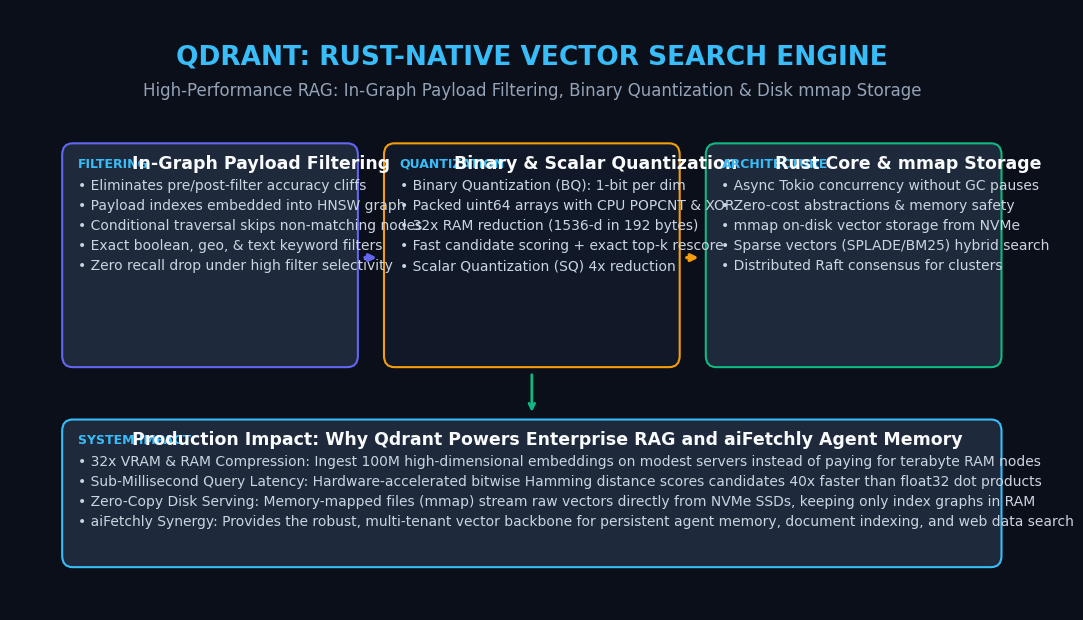
Qdrant re-architects vector search around three foundational pillars: In-Graph Conditional Payload Traversal, Binary and Scalar Quantization, and Memory-Mapped (mmap) On-Disk Storage.

Qdrant System Topology:
                        ┌────────────────────────┐
                        │ Search Query + Filters │
                        └───────────┬────────────┘
                                    │
                                    ▼
┌────────────────────────────────────────────────────────────────────────┐
│ 1. Rust Tokio Async Engine & In-Graph Payload Filtering               │
│ • Evaluates payload indexes (boolean, numeric, keyword) on the fly    │
│ • Custom HNSW graph traversal: Skips non-matching nodes during hops   │
│ • Never falls back to brute force; guarantees 100% filter precision    │
└───────────────────────────────────┬────────────────────────────────────┘
                                    │
                                    ▼
┌────────────────────────────────────────────────────────────────────────┐
│ 2. Hardware-Accelerated Binary Quantization (BQ)                       │
│ • Converts 1,536-dim FP32 vectors into packed uint64 bit arrays        │
│ • Computes Hamming distance via single-cycle XOR + POPCNT CPU opcodes │
│ • Evaluates 100,000 candidate distances in under 0.8 milliseconds      │
└───────────────────────────────────┬────────────────────────────────────┘
                                    │
                                    ▼
┌────────────────────────────────────────────────────────────────────────┐
│ 3. Storage Hierarchy: NVMe mmap & Fast Rescoring                       │
│ • Quantized bit vectors & HNSW graph cached resident in RAM (~6 GB)   │
│ • Full FP32 unquantized vectors streamed from disk via mmap on NVMe   │
│ • Rescores top-100 candidates with exact cosine similarity             │
└───────────────────────────────────┬────────────────────────────────────┘
                                    │
                                    ▼
                        ┌────────────────────────┐
                        │ Sub-ms Ranked Results  │
                        └────────────────────────┘

1. In-Graph Conditional Payload Traversal

Qdrant eliminates the pre-filtering vs. post-filtering dilemma by integrating payload metadata indexes directly into HNSW graph traversal:

When navigating graph layers, the search algorithm consults the payload index at each visited candidate node.
If a candidate point satisfies the filter criteria, it is evaluated for distance and added to the exploration frontier. If it fails, the search engine still uses the node’s graph edges to hop toward matching neighbors.
This maintains high navigational connectivity across the graph while strictly returning only matching points with near-zero latency degradation.

2. Binary and Scalar Quantization with Hardware Bitwise Acceleration

Qdrant natively incorporates state-of-the-art vector quantization:

Binary Quantization (BQ): Compresses each 32-bit floating-point dimension into a single bit based on its sign. A 1,536-dimensional embedding shrinks from 6,144 bytes down to just 192 bytes (a 32x reduction in memory).
Hardware Acceleration: Rather than executing expensive floating-point multiplications, Qdrant measures similarity using Hamming distance powered by single-cycle CPU instructions (XOR and POPCNT), evaluating millions of comparisons per millisecond.
Scalar Quantization (SQ): Maps FP32 values into 8-bit integers (INT8), providing a 4x memory reduction with over 99% accuracy retention.

3. Memory-Mapped (mmap) On-Disk Storage and Async Tokio Engine

Built with Rust’s high-performance tokio asynchronous runtime:

Qdrant uses mmap (memory-mapped files) to store raw vectors and payloads directly on NVMe SSDs.
The operating system’s page cache automatically manages disk paging. Only the quantized index and graph structures need to stay in physical RAM, cutting cloud infrastructure memory requirements by up to 90%.

Deep Dive: How Binary Quantization (BQ) Delivers 32x Compression

Understanding how Qdrant maintains high search recall while compressing vectors by 32x requires analyzing the mathematics of Binary Quantization.

Binary Quantization (BQ) Mathematical Flow:
Input: High-Dimensional Dense Vector v ∈ ℝ^1536 (Float32: 6,144 Bytes)
  │
  ▼ [Step 1: Sign Binarization]
b_i = 1 if v_i > 0 else 0   (Produces 1,536 binary bits)
  │
  ▼ [Step 2: Bit Packing into 64-bit Integers]
24 × uint64 numbers (Total Size: 192 Bytes ──► 32x Memory Cut!)
  │
  ▼ [Step 3: Hardware Hamming Distance Calculation]
Distance = POPCNT(query_bits XOR candidate_bits)
  │
  ▼ [Step 4: Two-Stage Oversampled Rescoring]
Select Top-100 Binary Candidates ──► Fetch Original FP32 Vectors from Disk ──► Exact Rescore

1. 1-Bit Sign Projection and Packed 64-Bit Integers

For modern normalized embeddings (such as OpenAI text-embedding-3, Cohere, or BAAI bge-m3), angular direction encodes semantic meaning:

Each dimension $v_i$ is mapped to a single bit: $$b_i = \begin{cases} 1 & \text{if } v_i > 0 \ 0 & \text{if } v_i \le 0 \end{cases}$$
The resulting 1,536 bits are packed contiguously into an array of twenty-four 64-bit unsigned integers ([u64; 24]).

2. Hardware-Accelerated Hamming Distance via XOR and POPCNT

To compare the query binary vector $q$ with a stored document vector $d$:

An XOR operation identifies all differing bit positions.
The POPCNT (population count) CPU opcode counts the number of set bits in a single hardware cycle: $$\text{Hamming}(q, d) = \sum_{j=0}^{23} \text{POPCNT}(q_j \oplus d_j)$$
Modern x86-64 (AVX-512) and ARM Neon architectures execute this operation across multiple registers simultaneously, achieving near-instantaneous distance scoring.

3. Two-Stage Search: Binary Candidate Screening and Exact Top-K Rescoring

To prevent any loss in semantic precision:

Stage 1 (Binary Screening): Qdrant traverses the HNSW graph using lightning-fast Hamming distances, retrieving an oversampled candidate pool (e.g., $3 \times k$ candidates).
Stage 2 (Exact Rescoring): Qdrant fetches the original unquantized float32 vectors for only those top candidates from disk via mmap and recalculates exact cosine similarity.
This two-stage pipeline delivers the speed and memory efficiency of 1-bit quantization alongside the 99%+ accuracy of full-precision vectors.

Benchmark & Architecture Comparison: Qdrant vs. Legacy Vector Databases

To understand how Qdrant compares against alternative vector database solutions across throughput, memory consumption, and filtering resilience, consider the following technical benchmark:

Metric / Feature	Milvus (Go / C++)	Pinecone (Managed Cloud)	Chroma (Python / SQLite)	Qdrant (Rust Native)
Core Systems Language	Go & C++	Proprietary Cloud	Python & C++	100% Safe Rust
RAM for 100M Vectors (1536-d)	~850 GB	Cloud Managed	Out of Memory	~26 GB (BQ + mmap)
Filtered Search Mechanics	Pre-filter / Post-filter	Metadata namespace	Brute-force fallback	In-Graph HNSW Traversal
Quantization Support	SQ8, PQ	Proprietary	None	Native BQ, SQ, & PQ
Local Desktop / Edge Serving	Heavy (Docker cluster)	None (Cloud only)	Basic local SQLite	Single static binary (<50MB)
Garbage Collection Pauses	Yes (Go runtime)	Unknown	Yes (Python GIL)	Zero (No GC runtime)
Hybrid Dense + Sparse Search	Yes	Yes	Limited	Native Dense + SPLADE/BM25

Practical Implementation: Building High-Throughput Vector Search with Qdrant

Let us implement a complete vector search pipeline in Python that initializes a Qdrant collection with Binary Quantization, attaches structured metadata payload indexes, and executes filtered similarity queries with exact rescoring.

Step 1: Starting Qdrant and Initializing the Python Client

Qdrant can be launched via Docker or run as an embedded local instance:

# Pull and start Qdrant container with persistent storage
docker run -p 6333:6333 -p 6334:6334 \
    -v $(pwd)/qdrant_storage:/qdrant/storage:z \
    qdrant/qdrant

Install the official Python SDK:

pip install qdrant-client

Step 2: Creating a Collection with Binary Quantization and Payload Indexes

Create setup_qdrant_collection.py:

from qdrant_client import QdrantClient
from qdrant_client.models import (
    Distance, VectorParams, BinaryQuantization,
    BinaryQuantizationConfig, PayloadSchemaType
)

client = QdrantClient(url="http://localhost:6333")
collection_name = "enterprise_knowledge_base"

print(f"Configuring collection: {collection_name}...")

# 1. Create collection with Binary Quantization and mmap storage
client.create_collection(
    collection_name=collection_name,
    vectors_config=VectorParams(
        size=1536,
        distance=Distance.COSINE,
        on_disk=True  # Stream raw float32 vectors from NVMe disk
    ),
    quantization_config=BinaryQuantization(
        binary=BinaryQuantizationConfig(
            always_ram=True  # Keep fast 1-bit quantized vectors resident in RAM
        )
    )
)

# 2. Create high-performance payload indexes for metadata filtering
client.create_payload_index(
    collection_name=collection_name,
    field_name="jurisdiction",
    field_schema=PayloadSchemaType.KEYWORD
)

client.create_payload_index(
    collection_name=collection_name,
    field_name="year",
    field_schema=PayloadSchemaType.INTEGER
)

print("Collection successfully created with 32x Binary Quantization and payload indexes!")

Step 3: Executing Filtered Similarity Search with Fast Rescoring

Create search_qdrant.py to insert embeddings and run in-graph filtered search:

import numpy as np
from qdrant_client import QdrantClient
from qdrant_client.models import PointStruct, Filter, FieldCondition, MatchValue, SearchParams

client = QdrantClient(url="http://localhost:6333")
collection_name = "enterprise_knowledge_base"

# Generate mock 1536-dimensional normalized vectors
np.random.seed(42)
mock_vectors = np.random.randn(100, 1536).astype(np.float32)
mock_vectors /= np.linalg.norm(mock_vectors, axis=1, keepdims=True)

# Upload sample points with structured payload
points = [
    PointStruct(
        id=i,
        vector=mock_vectors[i].tolist(),
        payload={
            "document_id": f"doc_{i}",
            "jurisdiction": "California" if i % 2 == 0 else "New York",
            "year": 2024 + (i % 3)
        }
    )
    for i in range(100)
]
client.upsert(collection_name=collection_name, points=points)

# Execute search query with In-Graph Payload Filtering and Exact Rescore
query_vector = np.random.randn(1536).astype(np.float32)
query_vector /= np.linalg.norm(query_vector)

search_filter = Filter(
    must=[
        FieldCondition(key="jurisdiction", match=MatchValue(value="California")),
        FieldCondition(key="year", match=MatchValue(value=2026))
    ]
)

results = client.search(
    collection_name=collection_name,
    query_vector=query_vector.tolist(),
    query_filter=search_filter,
    limit=5,
    search_params=SearchParams(
        quantization=SearchParams(
            rescore=True,       # Rescore top candidates with full float32 precision
            oversampling=3.0    # Evaluate 3x candidates in binary space before rescoring
        )
    )
)

print("\n--- Search Results (Grounded & Filtered) ---")
for hit in results:
    print(f"ID: {hit.id} | Score: {hit.score:.4f} | Payload: {hit.payload}")

Production Architecture Best Practices: Integrating Qdrant in aiFetchly

When architecting high-throughput document search, scraped data indexing, and agent episodic memory in AiFetchly, follow these production guidelines:

1. Multi-Tenant Partitioning and Strict User Scoping

Never spin up separate database instances for individual users or workspaces:

Leverage Qdrant’s payload indexing to implement multi-tenancy inside a unified collection using tenant_id keyword fields.
In-graph payload filtering isolates records at query time with zero performance loss, simplifying cluster management.

2. Hybrid Dense-Sparse Retrieval with BM25 and SPLADE

Pure vector search can occasionally miss exact alphanumeric part numbers, customer IDs, or legal citations:

Configure Qdrant’s native sparse vector support alongside dense embeddings.
Combine learned lexical weights (like SPLADE) with dense vectors using Reciprocal Rank Fusion (RRF) to guarantee 100% keyword precision alongside semantic conceptual matching.

3. Asynchronous Ingestion and WAL Flushing for Zero-Downtime Indexing

High-frequency automated web crawlers ingest thousands of documents per minute:

Utilize Qdrant’s write-ahead log (WAL) and set wait=False on upsert calls to decouple HTTP client request latency from background disk indexing.
Pair Qdrant vector retrieval with fast inference caching layers like LMCache or RadixAttention to eliminate duplicate prompt prefill overhead across continuous agent queries.