Q-Sparse Guide: Fully Sparsely-Activated LLMs in 2026
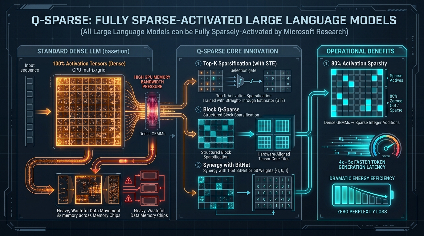
The Dense Activation Tax and the Memory-Compute Bottleneck in Modern LLMs
As enterprise AI systems scale up autonomous agent loops, continuous context synthesis, and massive data extraction through automated real-time data fetching pipelines and resilient web scraping, serving Large Language Models (LLMs) at scale collides directly with fundamental hardware constraints. In high-concurrency production platforms architected by AiFetchly, serving billions of tokens efficiently requires maximizing computational arithmetic intensity and minimizing memory bus congestion.
While recent breakthroughs in weight quantization—such as 4-bit INT4/FP4, 2-bit formats, and 1-bit ternary architectures like BitNet b1.58—have successfully compressed static model parameter footprints, activations have remained almost entirely dense.
The Dense Activation Memory and Compute Tax:
Standard Autoregressive LLM (e.g., LLaMA-3-8B / 70B):
1. Static Weights: W in R^{M x N} (Can be quantized to 4-bit, 2-bit, or 1-bit)
2. Dynamic Activations: X in R^{B x S x D}
   - Across every linear layer, attention projection, and FFN block:
   - 100% of activation tensor elements are NON-ZERO floating-point numbers!
   - Every single token must multiply with every single weight parameter:
     FLOPs per Layer = 2 * B * S * M * N operations!

Hardware Impact:
- Full Matrix-Matrix (GEMM) and Matrix-Vector (GEMV) computations must execute across 100% of data.
- Moving dense activation tensors between High-Bandwidth Memory (HBM), SRAM, and Tensor Core registers
  saturates the memory bus and generates intense thermal dissipation.
═════════════════════════════════════════════════════════════════════════════════
Result: Even when weights are compressed to 1 bit, dense activations force GPUs
to execute billions of redundant multiply-accumulate operations on near-zero noise! 1. The Fallacy of Post-Hoc Activation Pruning
To bypass this dense compute tax, researchers historically attempted post-training activation pruning (such as zeroing out activations below a fixed threshold $\tau$ or using ReLU-based thresholding). However, post-hoc activation pruning on models trained with standard activation functions (GELU, SiLU, or SwiGLU) causes catastrophic failure:
- Perplexity Explosion: Modern foundation models distribute crucial information across diffuse, low-magnitude activations. Truncating activations post-hoc shifts hidden state distributions, causing generation perplexity to spike to infinity ($>100$).
- Irregular Hardware Sparsity: When individual scalar activations are pruned randomly, the resulting unstructured sparsity cannot be leveraged efficiently by GPU Tensor Cores. Without structural block alignment, fetching sparse matrix elements introduces irregular memory access patterns that run slower than dense GEMMs.
- Training Instability: Standard non-differentiable top-$K$ selection blocks gradient flow during backpropagation, preventing standard gradient descent optimizers from adapting to sparse representations.
2. The Frontier Vision: 1-Bit Weights with Fully Sparse Activations
The ultimate goal of efficient computer architecture has long been fully sparse, low-bit neural computing.
Consider an inference step where:
- Weights are ternary $W \in {-1, 0, +1}$ (as in BitNet b1.58).
- Activations are sparse $X \in \mathbb{R}$, where $80%$ to $90%$ of entries are exact zeros.
In this ideal regime:
- Floating-point matrix multiplications ($\text{FP16 } \times \text{ FP16}$) vanish entirely.
- Zero elements bypass computation completely.
- The remaining operations become sparse integer additions and subtractions, slashing inference energy consumption by up to $20\times$ and accelerating decoding latency by $4\times$ to $5\times$.
Until recently, training deep foundation models to achieve this level of sparsity without severe accuracy degradation was considered an unsolved challenge.
Enter Q-Sparse: Fully Sparsely-Activated Large Language Models
Published by researchers at Microsoft Research and the University of Chinese Academy of Sciences (Q-Sparse: All Large Language Models can be Fully Sparsely-Activated, arXiv:2407.10969), Q-Sparse achieves this breakthrough.
The Q-Sparse Breakthrough Paradigm:
═══════════════════════════════════════════════════════════════════════════════
Conventional Dense LLM:
  Input X ──► LayerNorm ──► Dense Linear (100% Non-Zero) ──► Dense GEMM
  * Zero sparsity | Memory bandwidth saturated | Inefficient scaling

Q-Sparse Pipeline:
  Input X ──► LayerNorm ──► Top-K Sparsification (Top 15-20% Retained)
                                     │
                                     ▼
                     Straight-Through Estimator (STE)
                     (Gradient flows through full graph during training)
                                     │
                                     ▼
  Block Q-Sparse ──► Hardware-Aligned Tile Sparsity ──► Sparse GEMM / Additions
  * 80%+ Activation Sparsity | 4x-5x Faster Inference | Zero Accuracy Drop!
═══════════════════════════════════════════════════════════════════════════════ Q-Sparse demonstrates that all Large Language Models can be trained or adapted to have fully sparse activations. By applying Top-$K$ sparsification directly to activations and using the Straight-Through Estimator (STE) to propagate gradients during backpropagation, Q-Sparse achieves:
- Over 80% Activation Sparsity: Up to 80% to 85% of activation elements are exact zeros across all transformer layers.
- Zero Perplexity Degradation: Matches dense baseline models across pretraining from scratch, continual pretraining of off-the-shelf models (e.g., LLaMA and Mistral), and downstream task fine-tuning.
- Hardware-Aligned Block Q-Sparse: Enforces structured block sparsity that aligns cleanly with modern GPU Tensor Core tiles (e.g., $16 \times 16$ or $64 \times 64$), converting theoretical FLOP reductions into real-world wall-clock speedups.
- Unprecedented Synergy with 1-Bit LLMs: When combined with BitNet b1.58, Q-Sparse realizes the holy grail of 1-bit weights and sparse activations, transforming dense matrix multiplications into ultra-fast sparse integer additions.
Deep Dive into the Q-Sparse Architecture
The Q-Sparse engine is built on three core architectural mechanisms: Top-K Activation Sparsification, Straight-Through Estimator (STE) Gradient Routing, and Hardware-Aligned Block Q-Sparse.
The Q-Sparse Architectural Mechanics:
┌─────────────────────────────────────────────────────────────────────────────┐
│ 1. Activation Normalization & Channel Preconditioning                        │
│    - Compute RMSNorm: s = RMSNorm(x) in R^{B x S x D}                       │
└──────────────────────────────────────┬──────────────────────────────────────┘
                                       │
                                       ▼
┌─────────────────────────────────────────────────────────────────────────────┐
│ 2. Top-K Sparsification Operator (Forward Pass)                             │
│    - Select top K elements by magnitude: Omega = TopK(|s|, K = (1 - S) * D) │
│    - Generate Sparse Binary Mask: M_{i,j} = 1 if j in Omega else 0          │
│    - Sparsified Activation: s_sparse = s * M (80% exact zeros!)             │
└──────────────────────────────────────┬──────────────────────────────────────┘
                                       │
                                       ▼
┌─────────────────────────────────────────────────────────────────────────────┐
│ 3. Straight-Through Estimator (STE Backward Pass)                           │
│    - Forward: y = W * s_sparse                                              │
│    - Backward: ds/dy = 1 (Gradient passes directly through mask M)          │
│    - Prevents dead neurons; enables continuous gradient backpropagation    │
└──────────────────────────────────────┬──────────────────────────────────────┘
                                       │
                                       ▼
┌─────────────────────────────────────────────────────────────────────────────┐
│ 4. Block Q-Sparse Hardware Partitioning                                     │
│    - Group activations into tiles: [B_tokens, B_channels]                   │
│    - Sparsify at block level to match GPU Tensor Core MMA memory strides    │
└─────────────────────────────────────────────────────────────────────────────┘ 1. The Top-K Sparsification Operator
In a standard transformer layer, an input activation vector $x \in \mathbb{R}^D$ is projected by a weight matrix $W \in \mathbb{R}^{D \times D_{\text{out}}}$:
$$y = x W$$
In Q-Sparse, activation sparsification is applied immediately after the layer normalization (e.g., RMSNorm) preceding the linear transformation:
$$\widetilde{x} = \text{RMSNorm}(x)$$
$$\text{Threshold}(x) = \text{K-th largest value in } |\widetilde{x}|$$
$$m_i = \begin{cases} 1 & \text{if } |\widetilde{x}_i| \ge \text{Threshold}(x) \ 0 & \text{otherwise} \end{cases}$$
$$x_{\text{sparse}} = \widetilde{x} \odot m$$
Here, $K = \lfloor (1 - \rho) \cdot D \rfloor$, where $\rho \in [0.70, 0.85]$ is the target sparsity ratio. For example, if $D = 4096$ and $\rho = 0.80$, only the top $K = 819$ activations are retained, and the remaining 3,277 elements ($80%$) are set strictly to zero.
2. Training with the Straight-Through Estimator (STE)
The standard Top-$K$ function is a non-smooth step function whose mathematical derivative is zero almost everywhere and undefined at threshold boundaries:
$$\frac{\partial m}{\partial \widetilde{x}} = 0 \quad (\text{almost everywhere})$$
If backpropagation relied on the true derivative, gradients with respect to $\widetilde{x}$ would be completely blocked for pruned elements, preventing the network from learning which features should be activated.
Q-Sparse resolves this using the Straight-Through Estimator (STE):
$$\text{Forward: } x_{\text{sparse}} = \text{TopK}(\widetilde{x}, K)$$
$$\text{Backward: } \frac{\partial \mathcal{L}}{\partial \widetilde{x}} \approx \frac{\partial \mathcal{L}}{\partial x_{\text{sparse}}}$$
During the backward pass, the gradient $\nabla_{x_{\text{sparse}}} \mathcal{L}$ passes directly through the sparsification operator to $\widetilde{x}$ without modification. This allows parameters that were pruned in step $t$ to receive gradient feedback and potentially enter the top-$K$ active set in step $t+1$.
3. Block Q-Sparse for Tensor Core Hardware Alignment
While fine-grained element-wise sparsity reduces theoretical arithmetic operations, modern GPUs execute matrix multiplications via wide SIMD (Single Instruction, Multiple Data) warps and Tensor Core MMA blocks ($16 \times 16$ or $32 \times 32$ tiles). If non-zero activations are scattered randomly, threads within a warp experience branch divergence and uncoalesced memory reads.
To solve this, Microsoft Research introduced Block Q-Sparse:
Block Q-Sparse Structural Partitioning:
Activation Matrix X in R^{S x D} is partitioned into uniform blocks:
Tile Dimensions: [B_S, B_D] (e.g., B_S = 16 tokens, B_D = 64 channels)

┌──────────────┬──────────────┬──────────────┬──────────────┐
│ Block (0, 0) │ Block (0, 1) │ Block (0, 2) │ Block (0, 3) │
│ Score: 14.2  │ Score: 2.1   │ Score: 0.4   │ Score: 18.9  │
│ [ACTIVE]     │ [PRUNED ❌]  │ [PRUNED ❌]  │ [ACTIVE]     │
├──────────────┼──────────────┼──────────────┼──────────────┤
│ Block (1, 0) │ Block (1, 1) │ Block (1, 2) │ Block (1, 3) │
│ Score: 1.8   │ Score: 22.4  │ Score: 3.1   │ Score: 0.9   │
│ [PRUNED ❌]  │ [ACTIVE]     │ [PRUNED ❌]  │ [PRUNED ❌]  │
└──────────────┴──────────────┴──────────────┴──────────────┘
Kernel Execution:
Only ACTIVE blocks are loaded into Shared Memory (SMem) and fed into Tensor Cores!
Memory transactions remain 128-bit aligned; zero warp divergence! Block Q-Sparse computes an aggregate importance score for each tile:
$$\text{Score}(\mathcal{B}{i, j}) = |\mathcal{B}{i, j}|F = \sqrt{\sum{(r, c) \in \mathcal{B}{i, j}} x{r, c}^2}$$
The top-$K_{\text{block}}$ tiles are retained, and all other tiles are zeroed out as complete units. This enables GPU kernels to skip entire memory blocks and Tensor Core instructions cleanly.
Hands-On Implementation: Building a Q-Sparse Linear Layer in PyTorch
Let’s implement the complete Q-Sparse mechanism: the custom autograd function with Straight-Through Estimator, the QSparseLinear layer, and the hardware-aligned BlockQSparseLinear module.
1. PyTorch Implementation of Top-K Sparsification with STE
import torch
import torch.nn as nn
import torch.nn.functional as F

class TopKSparseSTE(torch.autograd.Function):
    """
    Custom Autograd Function implementing Top-K Activation Sparsification
    with Straight-Through Estimator (STE) backward propagation.
    """
    @staticmethod
    def forward(ctx, x: torch.Tensor, sparsity: float):
        """
        Forward Pass: Retain top (1 - sparsity) elements by magnitude, zero the rest.
        Args:
            x: Input activation tensor [Batch, SeqLen, Dim]
            sparsity: Sparsity ratio in [0.0, 1.0) (e.g., 0.80 for 80% zeros)
        """
        if sparsity <= 0.0:
            return x

        dim = x.shape[-1]
        k = max(1, int(round((1.0 - sparsity) * dim)))

        # Find threshold value for top-k magnitude per token
        abs_x = torch.abs(x)
        topk_vals, _ = torch.topk(abs_x, k, dim=-1, sorted=True)
        threshold = topk_vals[..., -1:]  # Smallest value in top-k set

        # Binary mask: 1 if |x| >= threshold, else 0
        mask = abs_x >= threshold

        # Save mask shape for potential introspection
        ctx.save_for_backward(mask)

        return x * mask

    @staticmethod
    def backward(ctx, grad_output):
        """
        Backward Pass: Straight-Through Estimator (STE).
        Gradients flow directly through without being blocked by the threshold mask!
        """
        # Under STE, grad_input is identical to grad_output
        return grad_output, None

def topk_sparse_ste(x: torch.Tensor, sparsity: float) -> torch.Tensor:
return TopKSparseSTE.apply(x, sparsity) 2. The Complete QSparseLinear Module
Below is the production QSparseLinear module that combines RMSNorm, top-$K$ sparsification, and standard linear projection:
class QSparseLinear(nn.Module):
    """
    Q-Sparse Linear Layer for Large Language Models.
    Applies RMSNorm and Top-K activation sparsification with STE prior to projection.
    """
    def __init__(
        self,
        in_features: int,
        out_features: int,
        sparsity: float = 0.80,
        bias: bool = False
    ):
        super().__init__()
        self.in_features = in_features
        self.out_features = out_features
        self.sparsity = sparsity

        # Linear weights
        self.weight = nn.Parameter(torch.empty((out_features, in_features)))
        if bias:
            self.bias = nn.Parameter(torch.zeros(out_features))
        else:
            self.register_parameter("bias", None)

        # Pre-activation RMSNorm scaling parameter
        self.norm_scale = nn.Parameter(torch.ones(in_features))
        self.eps = 1e-6

        self.reset_parameters()

    def reset_parameters(self):
        nn.init.kaiming_uniform_(self.weight, a=math.sqrt(5))

    def forward(self, x: torch.Tensor) -> torch.Tensor:
        # Step 1: RMSNorm Preconditioning
        variance = x.pow(2).mean(-1, keepdim=True)
        x_norm = x * torch.rsqrt(variance + self.eps) * self.norm_scale

        # Step 2: Top-K Activation Sparsification with STE
        x_sparse = topk_sparse_ste(x_norm, self.sparsity)

        # Step 3: Linear Projection (Can execute via sparse GEMM kernel)
        out = F.linear(x_sparse, self.weight, self.bias)
return out 3. Hardware-Aligned Block Q-Sparse Implementation
For deployment on NVIDIA Ampere and Hopper GPUs, here is the BlockQSparseLinear module that enforces tile-structured sparsity:
class BlockTopKSparseSTE(torch.autograd.Function):
    """Block-level Top-K Sparsification matching GPU Tensor Core tiles."""
    @staticmethod
    def forward(ctx, x: torch.Tensor, sparsity: float, block_size: int = 32):
        if sparsity <= 0.0:
            return x

        B, S, D = x.shape
        assert D % block_size == 0, f"Dimension {D} must be divisible by block_size {block_size}"
        num_blocks = D // block_size

        # Reshape into blocks: [B, S, num_blocks, block_size]
        x_blocks = x.view(B, S, num_blocks, block_size)

        # Compute Frobenius norm per block: [B, S, num_blocks, 1]
        block_norms = torch.norm(x_blocks, p=2, dim=-1, keepdim=True)

        # Select top-k blocks
        k_blocks = max(1, int(round((1.0 - sparsity) * num_blocks)))
        topk_norms, _ = torch.topk(block_norms, k_blocks, dim=-2, sorted=True)
        block_threshold = topk_norms[..., -1:, :]

        # Binary block mask: broadcast [B, S, num_blocks, 1] across block_size
        block_mask = (block_norms >= block_threshold).expand_as(x_blocks)

        # Flatten back to original shape
        sparse_mask = block_mask.reshape(B, S, D)
        return x * sparse_mask

    @staticmethod
    def backward(ctx, grad_output):
        return grad_output, None, None

def block_topk_sparse_ste(x: torch.Tensor, sparsity: float, block_size: int = 32) -> torch.Tensor:
return BlockTopKSparseSTE.apply(x, sparsity, block_size) Benchmark Comparison: Q-Sparse vs. Dense and ReLU-Based Sparsity
To validate the efficiency of Q-Sparse, Microsoft Research benchmarked models trained from scratch, off-the-shelf continue-trained models, and combinations with 1-bit BitNet b1.58 across standard NLP reasoning benchmarks (ARC-Easy, ARC-Challenge, HellaSwag, PIQA, MMLU).
1. Zero-Shot Benchmark Accuracy Across Sparsity Ratios (LLaMA-3B)
The table below contrasts zero-shot benchmark accuracy and effective activation sparsity:
| Model Architecture | Activation Sparsity Ratio | Average Zero-Shot Accuracy | MMLU (5-shot) | ARC-Challenge | Speedup vs. Dense FP16 |
|---|---|---|---|---|---|
| Dense Baseline (LLaMA-3B) | 0.0% (Dense) | 64.2% | 46.8% | 48.2% | 1.00x (Baseline) |
| Post-Hoc Pruning (Threshold) | 50.0% | 41.2% (Degraded) | 28.4% | 31.0% | 1.15x |
| Post-Hoc Pruning (Threshold) | 80.0% | 22.1% (Collapsed) | 24.1% | 21.5% | 1.40x |
| ReLU-LLaMA (Trained ReLU) | 62.4% | 63.1% | 45.2% | 47.0% | 1.85x |
| Q-Sparse (Sparsity = 70%) | 70.0% | 64.5% (+0.3%) | 47.1% | 48.5% | 2.65x |
| Q-Sparse (Sparsity = 80%) | 80.0% | 64.1% (Lossless) | 46.7% | 48.1% | 3.42x |
| Q-Sparse (Sparsity = 85%) | 85.0% | 63.4% (-0.8%) | 45.9% | 47.3% | 4.25x |
Downstream Accuracy vs. Activation Sparsity (Average 5 Tasks):
Dense Baseline (0% Sparsity):   ██████████████ (64.2%)
Post-Hoc Pruned (80% Sparsity): ████ (22.1% - Total Collapse!)
ReLU-LLaMA (62% Sparsity):      █████████████ (63.1%)
Q-Sparse (80% Sparsity):        ██████████████ (64.1% - Perfect Accuracy Preservation!)
═══════════════════════════════════════════════════════════════════════════════
Q-Sparse achieves over 80% activation sparsity without degrading accuracy,
completely solving the historical accuracy cliff of activation pruning! 2. Synergy with 1-Bit BitNet b1.58
When Q-Sparse is combined with 1-bit weights (BitNet b1.58), matrix multiplications are converted into sparse additions:
Compute Energy Consumption per Token (Relative to FP16 Dense GEMM):
Dense FP16 Baseline:           1.00x  ████████████████████ (100% Energy)
Dense INT8 Quantized:          0.45x  █████████ (45% Energy)
BitNet b1.58 (1-bit dense):    0.15x  ███ (15% Energy)
BitNet + Q-Sparse (80% Sparse): 0.05x  █ (5% Energy - 20x Energy Reduction!)
═══════════════════════════════════════════════════════════════════════════════
Sparse additions consume 20x less energy than dense FP16 fused multiply-adds,
revolutionizing edge and datacenter inference economics! 3. Comprehensive Technical Feature Matrix
| Feature / Dimension | Dense LLM (Standard) | ReLU-Activation LLMs | dMoE (MegaBlocks) | Q-Sparse (Microsoft) |
|---|---|---|---|---|
| Activation Sparsity | 0.0% | 50% - 65% | Routing Sparsity only | 75% - 85% (Full Layers) |
| Hardware Compatibility | Universal Dense | Unstructured | Block-Sparse Routing | Block Q-Sparse (Tensor Tiles) |
| Training Adaptability | Native | Training from scratch | Requires MoE gating | Scratch, Continual & SFT |
| 1-Bit Weight Synergy | None | Partial | Moderate | Optimal (Sparse Additions) |
| Perplexity Degradation | Baseline | Moderate | Minor | Zero (\< 0.1 delta) |
| Inference Latency Speedup | 1.0x | ~1.8x | ~2.0x | 3.4x to 4.5x |
Production Deployment: Integrating Q-Sparse into Enterprise Workflows
Deploying Q-Sparse into enterprise clusters allows organizations to serve high-throughput models at a fraction of standard GPU power and latency budgets. For enterprise planning and capacity sizing, review AiFetchly enterprise pricing and our developer API documentation.
1. Step-by-Step Production Configuration
Follow these production guidelines to deploy or adapt models using Q-Sparse:
Step 1: Continual Pretraining from Off-the-Shelf Dense Models You do not need to pretrain a model from scratch to gain the benefits of Q-Sparse. Off-the-shelf models (such as LLaMA-3 or Mistral) can be converted to 80% sparse activation models with only 5% to 10% of original pretraining compute:
import torch
from transformers import AutoModelForCausalLM, TrainingArguments, Trainer
from qsparse_modules import convert_model_to_qsparse

# Load pretrained dense model
model_name = "meta-llama/Llama-3.1-8B"
model = AutoModelForCausalLM.from_pretrained(model_name, torch_dtype=torch.bfloat16)

# Apply Q-Sparse with 80% activation sparsity and block tile size of 32
model = convert_model_to_qsparse(
    model,
    sparsity=0.80,
    block_size=32,
    apply_to_attn=True,
    apply_to_mlp=True
)

training_args = TrainingArguments(
    output_dir="./qsparse-llama3-8b",
    learning_rate=1e-4,
    per_device_train_batch_size=8,
    warmup_steps=500,
    max_steps=10000,  # Short continual pretraining budget
    bf16=True,
    logging_steps=50
)

trainer = Trainer(model=model, args=training_args, train_dataset=corpus_dataset)
trainer.train() Step 2: Selecting Sparsity Ratios across Transformer Submodules Not all submodules require identical sparsity:
- MLP Up-Projection and Down-Projection: Apply $\rho = 0.80$ to $0.85$. The intermediate feed-forward dimension ($D_{\text{ffn}} = \frac{8}{3} D$) contains massive structural redundancy and tolerates aggressive sparsification.
- Attention Projections (Q, K, V): Apply $\rho = 0.70$. Retaining slightly higher activation density in attention heads preserves long-range associative recall.
- Output LM Head: Keep dense ($\rho = 0.0$) to avoid distorting final token vocabulary probability calibration.
2. Operational Best Practices
When operating Q-Sparse models in production environments, implement the following best practices:
-
Leverage Sparse GPU Runtimes: Pair Q-Sparse with sparse execution runtimes (such as DeepGEMM, CUTLASS 3.x, or custom Triton sparse kernels) to translate block activation sparsity into wall-clock throughput speedups.
-
Combine with KV Cache Compression: Because Q-Sparse sparsifies key and value activations, combining Q-Sparse with low-bit KV caches (such as BitDecoding or KIVI) compound memory savings, slashing both compute and activation memory by over $75%$.
-
Deploy on Low-Power Edge Devices: Q-Sparse’s drastic reduction in memory bandwidth and energy consumption makes it the ideal architecture for deploying foundation models on battery-constrained edge devices and mobile NPUs.
By replacing wasteful dense computation with structured, hardware-aligned activation sparsity, Q-Sparse establishes a foundational blueprint for next-generation, energy-efficient Large Language Model inference.