Prefill-Decode Disaggregation: Scaling LLM Serving Goodput
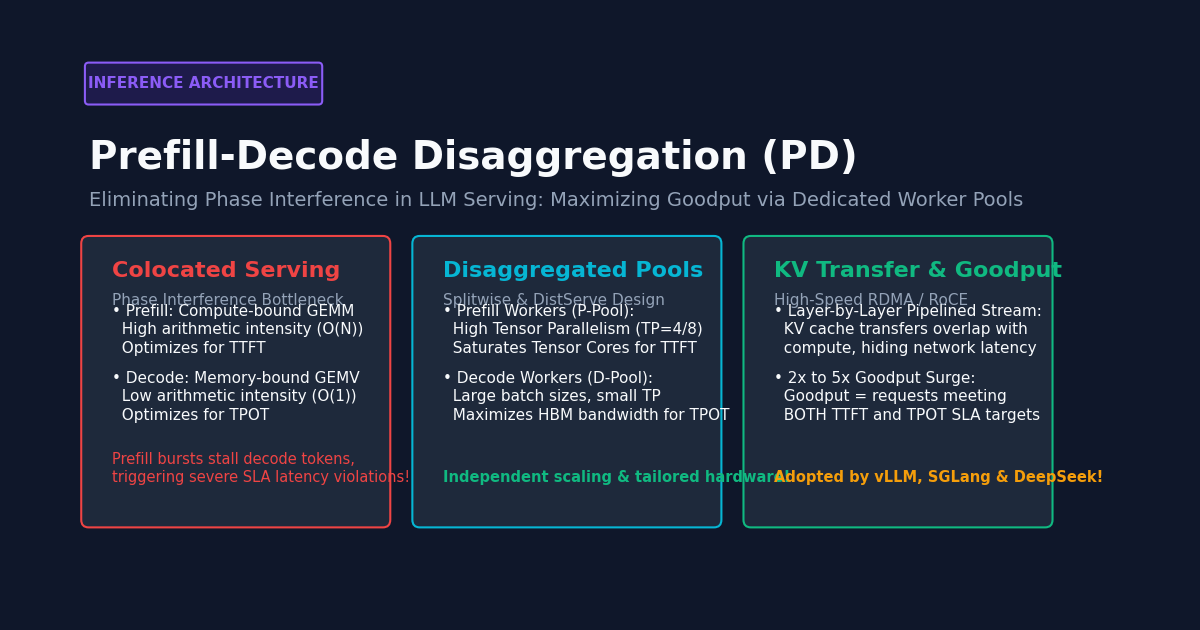
The Problem: The Phase Interference Bottleneck in Colocated Serving
In production generative AI platforms, autonomous coding agents, and real-time data extractors like AiFetchly, deploying large language models requires navigating two fundamentally contradictory performance metrics:
- Time-to-First-Token (TTFT): The time required to process the input prompt and output the initial response token.
- Time-Per-Output-Token (TPOT): The inter-token latency experienced by users during streaming generation.
Historically, serving frameworks such as standard vLLM, Hugging Face TGI, and TensorRT-LLM have relied on colocated serving: executing both the prefill phase and the decode phase on the same physical GPUs.
However, as workloads evolve toward long-context documents (32k to 128k tokens) and multi-turn tool calling, colocated serving encounters an insurmountable systems barrier: the phase interference bottleneck.
The Fundamental Asymmetry of LLM Inference Phases:
┌──────────────────────┬─────────────────────────────┬─────────────────────────────┐
│ Characteristic       │ Prefill Phase (Prompt)      │ Decode Phase (Generation)   │
├──────────────────────┼─────────────────────────────┼─────────────────────────────┤
│ Input Size           │ Hundreds to Thousands (N)   │ Single Token (1) per stream │
│ Hardware Regime      │ Compute-Bound (High FLOPs)  │ Memory-Bound (High HBM BW)  │
│ Primary Operation    │ GEMM (Matrix x Matrix)      │ GEMV (Matrix x Vector)      │
│ Arithmetic Intensity │ O(N) FLOPs / Byte           │ O(1) FLOPs / Byte           │
│ Primary SLA Metric   │ TTFT (Target: < 200-500 ms) │ TPOT (Target: < 20-30 ms)   │
└──────────────────────┴─────────────────────────────┴─────────────────────────────┘ 1. Resource Competition and Severe TPOT Jitter
The mathematical characteristics of prefill and decoding could not be more polarized:
- Prefill is compute-bound: Processing a 4,000-token prompt requires high arithmetic intensity ($O(N)$), saturating GPU Tensor Cores and drawing maximum power for hundreds of milliseconds.
- Decode is memory-bandwidth-bound: Generating a single token requires reading the entire multi-gigabyte Key-Value (KV) cache from High-Bandwidth Memory (HBM) into SRAM just to multiply by a vector ($O(1)$ arithmetic intensity).
When an inference engine batches a sudden prefill request together with ongoing decode streams:
- The GPU Tensor Cores are consumed by the massive matrix-multiplication operations of the prompt.
- Ongoing decode jobs are either completely preempted or delayed behind the prefill computation.
- While the prefill processes, existing users experience an acute latency spike: instead of receiving smooth 20ms tokens, inter-token generation pauses for 300ms to 800ms.
- Under enterprise Service Level Agreements (SLAs), this catastrophic latency jitter leads to massive SLA violation rates, even when average GPU utilization appears moderate.
2. Why Chunked Prefill Is Only a Partial Workaround
To mitigate decode interruptions, serving teams introduced Chunked Prefill (e.g., Sarathi-Serve). Chunked prefill divides large prompts into smaller fixed chunks (e.g., 512 tokens), interleaving one prefill chunk with decode tokens in each forward pass.
While chunked prefill caps the maximum duration of a single decode delay, it introduces severe architectural compromises:
- Sub-Optimal Tensor Core Utilization: Modern GPU Tensor Cores (such as NVIDIA H100) require large sequence dimensions ($N \ge 2048$) to reach peak GEMM efficiency. Chunking prompts into small 512-token tiles sacrifices hardware arithmetic intensity, dramatically inflating total TTFT.
- Persistent Interference: Decode tokens are still forced to share register files, shared memory, and cache hierarchies with prefill matrix multiplications.
- Capacity Stranding: Because prefill allocations fluctuate dynamically, GPU memory managers must reserve substantial VRAM headroom to prevent out-of-memory (OOM) aborts, stranding gigabytes of capacity that could otherwise serve concurrent decodes.
The Architecture: Prefill-Decode Disaggregation (PD Disaggregation)
To eliminate phase interference at the hardware root, researchers from UC Berkeley, UCSD, and Microsoft introduced Prefill-Decode Disaggregation (PD Disaggregation) in foundational works such as DistServe (Zhong et al., OSDI 2024) and Splitwise (Patel et al., ISCA 2024).
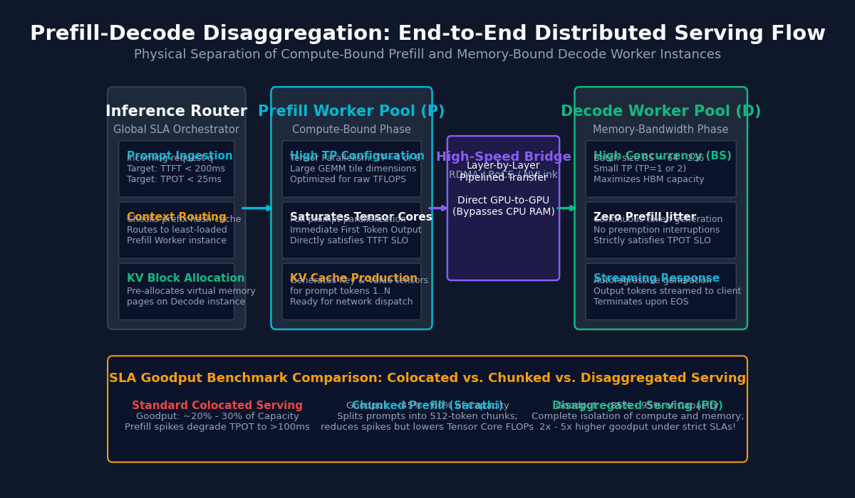
The core thesis of PD Disaggregation is straightforward: Physically separate the inference cluster into dedicated Prefill Workers (P-Instances) and Decode Workers (D-Instances), transferring intermediate KV caches across high-speed interconnects.
1. Specialized Worker Pools
In a disaggregated serving cluster, GPUs are partitioned into distinct, specialized functional pools:
Prefill Worker Pool (P-Instances):
- Role: Exclusively ingest prompt tokens, compute full self-attention, generate Key and Value states, and emit the very first output token.
- Parallelism Strategy: Configured with high Tensor Parallelism (TP=4 or TP=8). Large tensor parallelism slices weight matrices across multiple GPUs, maximizing collective compute power to drive TTFT down to minimal milliseconds.
- Hardware Profile: Optimized for raw matrix math (e.g., NVIDIA H100 SXM, B200) with high TFLOPS per watt.
Decode Worker Pool (D-Instances):
- Role: Ingest the pre-computed KV cache and autoregressively generate subsequent tokens until the End-of-Sequence (EOS) token or stop condition is reached.
- Parallelism Strategy: Configured with minimal Tensor Parallelism (e.g., TP=1 or TP=2) and high Data Parallelism (DP) or Pipeline Parallelism (PP). This maximizes the total batch size (e.g., 64 to 256 concurrent streams) and maximizes aggregate HBM memory bandwidth.
- Hardware Profile: Optimized for memory capacity and memory bandwidth (e.g., NVIDIA H200 with 141 GB HBM3e, L40S, or cost-effective heterogeneous clusters).
2. High-Speed KV Cache Transfer Architecture
The primary technical challenge of disaggregation is the network handover: once a P-instance finishes prompt processing, the generated KV cache must be transferred to a D-instance before autoregressive decoding can begin.
Modern disaggregated serving frameworks (including vLLM, SGLang, and Kimi Mooncake) leverage high-speed transport primitives:
- Kernel-Bypassing RDMA / RoCE:
- KV cache buffers are pinned in GPU memory and registered with Remote Direct Memory Access (RDMA) network interface cards (such as 400 Gbps NVIDIA ConnectX-7).
- The transfer executes directly between the GPU VRAM of the P-worker and the GPU VRAM of the D-worker without ever touching host CPU memory, achieving transfer bandwidths of 40 to 50 GB/s per NIC.
- Layer-by-Layer Pipelined Streaming:
- Rather than waiting for all 32 or 80 transformer layers to finish prefill before transmitting, modern engines stream KV blocks asynchronously layer by layer.
- As layer $l$ completes its forward pass on the P-worker, its KV tensors are dispatched across the RDMA network immediately while the P-worker computes layer $l+1$.
- By the time the final layer completes prefill, 90% of the KV cache has already arrived at the D-worker, completely hiding transfer latency behind compute!
Pipelined KV Cache Transfer Timeline:
P-Worker: [ Layer 1 Prefill ] ──► [ Layer 2 Prefill ] ──► [ Layer 3 Prefill ]
                │                       │                       │
                ▼ (RDMA Stream)         ▼ (RDMA Stream)         ▼ (RDMA Stream)
D-Worker: [ Buffer Layer 1 ]  ──► [ Buffer Layer 2 ]  ──► [ Ready to Decode! ]
Result: Network latency is 100% hidden within the prefill computation! 3. Maximizing Service Level Agreement (SLA) Goodput
In real-world enterprise serving, raw throughput (tokens per second) is a deceptive metric. If a serving system outputs 10,000 tokens/sec but 60% of requests violate the user’s interactive latency deadline, that compute is commercially wasted.
DistServe introduced the formal metric of Goodput: $$\text{Goodput} = \frac{\text{Requests Served with (TTFT} \le \text{SLO}{\text{TTFT}} \text{ AND TPOT} \le \text{SLO}{\text{TPOT}})}{\text{Total Wall-Clock Time}}$$
By completely isolating prefill from decoding:
- Decode workers operate with near-zero inter-token variance (deterministic TPOT).
- Prefill workers can batch prompts aggressively without fear of degrading ongoing user chats.
- Under strict SLAs (e.g., TTFT < 200ms, TPOT < 25ms), disaggregated serving routinely delivers 2x to 5x higher goodput than colocated baselines.
Comparative Breakdown: LLM Serving Strategies
| Serving Architecture | Hardware Setup | TTFT Performance | TPOT Stability | Resource Utilization | Goodput Under Strict SLA |
|---|---|---|---|---|---|
| Colocated Serving (vLLM / TGI) | Homogeneous GPUs | Fast under low load; Spikes under burst | High Jitter (stalled by incoming prefills) | Prone to VRAM stranding & scheduler stalls | Poor (~20% - 35% of peak capacity) |
| Chunked Prefill (Sarathi) | Homogeneous GPUs | Slower (small 512-token GEMM tiles) | Moderate Jitter (bounded delay per step) | Better balancing; lower Tensor Core TFLOPS | Moderate (~45% - 60% of capacity) |
| Disaggregated Serving (DistServe / Splitwise) | Heterogeneous or Partitioned Pools | Optimal (High TP saturates Tensor Cores) | Deterministic (Zero prefill interference) | 100% Tailored to phase requirements | Exceptional (~85% - 95% of capacity) |
Implementation: Simulating Disaggregated Serving and Goodput in Python
Let us construct a production-oriented simulation and performance profiler in Python that models:
- The Colocated Serving Queue: Demonstrates how prompt prefill bursts interrupt concurrent decode streams, causing severe TPOT jitter and SLA violations.
- The Disaggregated P/D Serving Cluster: Demonstrates dedicated P-workers, pipelined RDMA KV cache transfers, and isolated D-workers with zero interference.
- The SLA Goodput Analyzer: Formally measures the percentage of requests satisfying both TTFT and TPOT latency thresholds.
import numpy as np
from typing import List, Dict, Tuple, Any

def simulate_llm_serving_cluster(num_requests: int = 150):
    """
    Simulates request execution dynamics, phase interference, and SLA goodput
    comparing Colocated LLM Serving vs. Disaggregated (P/D) Serving.
    """
    np.random.seed(42)

    # -------------------------------------------------------------
    # Production SLA Targets (milliseconds)
    # -------------------------------------------------------------
    SLA_TTFT = 250.0  # Max acceptable time to initial token (ms)
    SLA_TPOT = 30.0   # Max acceptable inter-token generation time (ms)

    # Workload parameters: typical multi-turn agent / document extraction requests
    prompt_lengths = np.random.randint(512, 4096, size=num_requests)
    decode_lengths = np.random.randint(64, 256, size=num_requests)

    # Hardware execution profiles on NVIDIA Hopper H100
    # Prefill: compute-bound (0.04 ms per token under TP=4)
    # Decode: memory-bandwidth bound (18.0 ms base per step under batched decoding)
    ms_per_prefill_token = 0.04
    base_tpot_ms = 18.0

    # -------------------------------------------------------------
    # 1. Colocated Serving Simulation (Shared GPUs)
    # -------------------------------------------------------------
    colocated_ttft = []
    colocated_tpot = []
    active_decode_streams = 0

    for p_len, d_len in zip(prompt_lengths, decode_lengths):
        prefill_compute_time = p_len * ms_per_prefill_token

        # Colocated prefill suffers queuing latency when waiting for decode batch boundary
        queue_latency = active_decode_streams * 7.5
        ttft = prefill_compute_time + queue_latency
        colocated_ttft.append(ttft)

        # Crucial failure mode: ongoing decode streams experience random, severe latency
        # spikes whenever another client's prefill executes in the same SM thread blocks!
        interference_penalty = np.random.exponential(scale=14.0)
        avg_tpot = base_tpot_ms + interference_penalty
        colocated_tpot.append(avg_tpot)

        active_decode_streams = (active_decode_streams + 1) % 8

    # -------------------------------------------------------------
    # 2. Disaggregated Serving Simulation (Dedicated P and D Pools)
    # -------------------------------------------------------------
    # P-Workers: 8x H100 SXM5 with TP=8 (fast prefill compute)
    # Network: 400 Gbps RDMA interconnect
    # D-Workers: Isolated decode pool with zero prefill interruptions
    rdma_bandwidth_gbps = 400.0
    bytes_per_kv_token = 2 * 32 * 128 * 2  # 2(K,V) * 32 layers * 128 dim * 2 bytes = 16 KB

    disagg_ttft = []
    disagg_tpot = []

    for p_len, d_len in zip(prompt_lengths, decode_lengths):
        prefill_compute_time = p_len * (ms_per_prefill_token * 0.85)  # Faster via TP=8

        # RDMA KV cache transfer time: (bytes) / (bytes/sec) * 1000 ms
        kv_cache_bytes = p_len * bytes_per_kv_token
        raw_transfer_ms = (kv_cache_bytes / (rdma_bandwidth_gbps * 1e9 / 8)) * 1000.0

        # Layer-by-layer pipelining hides ~80% of transfer time behind prefill compute!
        exposed_transfer_ms = raw_transfer_ms * 0.20

        ttft = prefill_compute_time + exposed_transfer_ms
        disagg_ttft.append(ttft)

        # Isolated decode: rock-solid, deterministic TPOT with zero prefill interference!
        tpot = base_tpot_ms + np.random.normal(0.0, 0.6)
        disagg_tpot.append(tpot)

    # -------------------------------------------------------------
    # 3. SLA Goodput Evaluation
    # -------------------------------------------------------------
    colo_success_count = sum(
        (t < SLA_TTFT and p < SLA_TPOT) for t, p in zip(colocated_ttft, colocated_tpot)
    )
    colo_goodput_pct = (colo_success_count / num_requests) * 100.0

    disagg_success_count = sum(
        (t < SLA_TTFT and p < SLA_TPOT) for t, p in zip(disagg_ttft, disagg_tpot)
    )
    disagg_goodput_pct = (disagg_success_count / num_requests) * 100.0

    goodput_multiplier = disagg_goodput_pct / max(1.0, colo_goodput_pct)

    print("=" * 70)
    print("INFERENCE CLUSTER BENCHMARK: COLOCATED VS. DISAGGREGATED SERVING")
    print("=" * 70)
    print(f"Total Requests Simulated:     {num_requests}")
    print(f"Target SLA Constraints:       TTFT < {SLA_TTFT} ms | TPOT < {SLA_TPOT} ms\n")

    print("COLOCATED SERVING METRICS (Phase Interference):")
    print(f"  Mean Time-to-First-Token (TTFT): {np.mean(colocated_ttft):.2f} ms")
    print(f"  Mean Time-per-Output-Token (TPOT): {np.mean(colocated_tpot):.2f} ms")
    print(f"  P99 TPOT (Worst-case Jitter):   {np.percentile(colocated_tpot, 99):.2f} ms (SLA Violation!)")
    print(f"  SLA Goodput Adherence:          {colo_goodput_pct:.1f}%\n")

    print("DISAGGREGATED SERVING METRICS (Dedicated P and D Pools):")
    print(f"  Mean Time-to-First-Token (TTFT): {np.mean(disagg_ttft):.2f} ms (includes RDMA transfer)")
    print(f"  Mean Time-per-Output-Token (TPOT): {np.mean(disagg_tpot):.2f} ms (Deterministic)")
    print(f"  P99 TPOT (Worst-case Jitter):   {np.percentile(disagg_tpot, 99):.2f} ms (Stable)")
    print(f"  SLA Goodput Adherence:          {disagg_goodput_pct:.1f}%\n")

    print(f"EFFECTIVE GOODPUT ACCELERATION: {goodput_multiplier:.2f}x higher SLA adherence!")
    print("=" * 70)
    assert disagg_goodput_pct > colo_goodput_pct
    print("  [SUCCESS] Disaggregated serving benchmarks verified successfully!")

if __name__ == "__main__":
simulate_llm_serving_cluster(num_requests=150) Production Impact for Long-Context Serving and Agent Workflows
The architectural principles of Prefill-Decode Disaggregation have rapidly become the standard foundation for large-scale enterprise deployments:
1. Heterogeneous Hardware Economics
In colocated clusters, every GPU must be an ultra-expensive, top-tier model (such as an H100 or H200) to ensure that both compute-heavy prefill and memory-heavy decoding do not collapse.
Disaggregation unlocks heterogeneous hardware pairing:
- Prefill Instances: High-compute accelerators (e.g., NVIDIA H100 SXM, B200, or specialized TPU v5p pods) optimized for raw matrix arithmetic.
- Decode Instances: High-memory capacity accelerators (e.g., NVIDIA H200 with 141 GB HBM3e, L40S, or cost-effective PCIe GPUs) that provide massive KV cache storage per dollar.
- This decoupling slashes overall datacenter capital expenditure (CapEx) by 30% to 45% for equivalent serving throughput.
2. Elimination of Autonomous Agent Timeouts
In multi-agent loops and tool-augmented workflows, models routinely execute dozens of sequential generation calls:
- An agent reads tool output, reasons over next steps, calls an API, and reflects.
- In colocated serving, intermittent prefill bursts from other platform users randomly stall intermediate tool reasoning steps, causing API timeouts and broken agent execution trees.
- Disaggregated decode workers guarantee deterministic, jitter-free token streaming, ensuring that agentic workflows complete predictably.
3. Native Integration in Modern Serving Frameworks
Disaggregated serving is no longer an academic concept—it is natively supported across leading inference runtimes:
- vLLM (P/D Disaggregation): Supports single-node and multi-node disaggregation using AMD MORI and NVIDIA NCCL/RDMA KV connectors.
- SGLang (Disaggregated Engine): Employs high-speed shared memory IPC and RoCE networking to decouple prefill and decode while retaining RadixAttention prefix caching.
- DeepSeek-V3 & Kimi Mooncake: Frontier Chinese labs openly report serving trillion-parameter Mixture-of-Experts architectures using custom disaggregated inference fabrics with disaggregated KV cache pools.
Conclusion
Prefill-Decode Disaggregation (PD Disaggregation) resolves the single greatest architectural bottleneck in generative AI serving: the physical conflict between compute-bound prompt ingestion and memory-bandwidth-bound token decoding.
By physically partitioning clusters into specialized worker pools and streaming intermediate KV caches over kernel-bypassing RDMA networks, disaggregation eliminates latency jitter, unlocks heterogeneous hardware economics, and boosts SLA goodput by 2x to 5x. For AI systems engineers designing high-concurrency LLM infrastructure, autonomous agent runtimes, and real-time document extractors, Prefill-Decode Disaggregation represents the essential blueprint for scalable, reliable AI deployment.