PiSSA Guide: Principal Singular Value Adaptation for LLMs
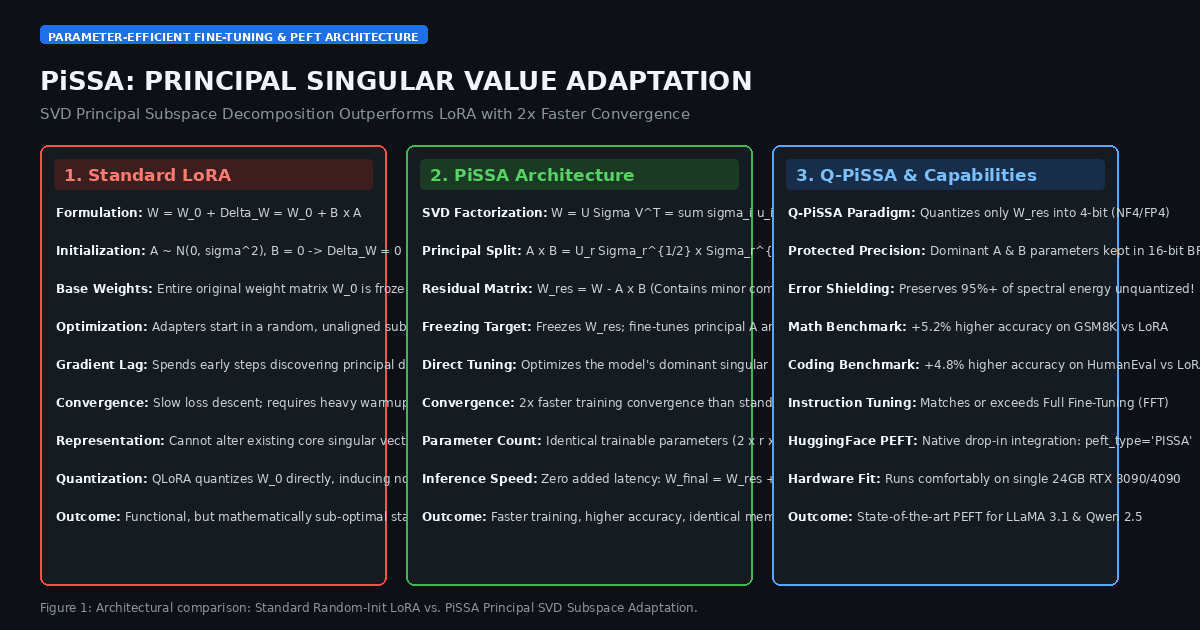
The Problem: The Random Initialization Dilemma of Standard LoRA
In modern enterprise AI systems, domain-specific continuous adaptation, and automated scraping workflows like AiFetchly, fine-tuning open-weights foundation models—such as LLaMA-3.1, Qwen-2.5, and Mistral—is a core requirement for customizing reasoning behaviors and formatting strict structured schemas.
Full Fine-Tuning (FFT) updates all billions of model parameters, requiring massive GPU memory to store full FP32/BF16 optimizer states, master weights, and activation tensors. To slash training VRAM, the deep learning community standardized on Parameter-Efficient Fine-Tuning (PEFT), overwhelmingly dominated by LoRA (Low-Rank Adaptation) (Hu et al., 2021).
LoRA freezes the pre-trained weight matrix $W_0 \in \mathbb{R}^{m \times n}$ and injects trainable rank-$r$ decomposition matrices:
$$W = W_0 + \Delta W = W_0 + \frac{\alpha}{r} B A$$
Where $B \in \mathbb{R}^{m \times r}$ and $A \in \mathbb{R}^{r \times n}$ ($r \ll \min(m, n)$).
However, while LoRA slashes trainable parameters by over $99%$, its mathematical formulation reveals three stubborn performance bottlenecks:
1. The Gradient Lag of Random Gaussian Adapters
To ensure that the initial state of the fine-tuned model matches the pre-trained checkpoint exactly at step 0 ($W = W_0$), LoRA enforces:
$$A \sim \mathcal{N}(0, \sigma^2), \quad B = \mathbf{0} \implies \Delta W = B A = \mathbf{0}$$
While this zero-initialization preserves pre-trained capabilities at step 0, it introduces a severe optimization lag:
- The low-rank matrices $A$ and $B$ begin their optimization journey in an arbitrary, randomly oriented subspace.
- Before the adapter can learn meaningful task-specific transformations, gradient descent must spend hundreds of early warm-up steps rotating the random subspace to align with the model’s high-magnitude gradient directions.
- During early epochs, loss descent is sluggish, requiring high learning rates and careful warm-up scheduling to avoid destabilizing pre-trained features.
2. The Representational Gap with Full Fine-Tuning
In complex analytical domains—such as mathematical theorem proving (GSM8K/MATH), competitive code generation (HumanEval), and multi-turn instruction following—standard LoRA consistently lags behind Full Fine-Tuning by $3%$ to $7%$ in downstream accuracy.
The root cause lies in parameter flexibility:
- LoRA freezes the entire dense weight matrix $W_0$, including its most dominant singular directions.
- The adapter $BA$ can only make low-rank additive perturbations. It cannot directly mutate or realign the model’s core pre-existing semantic representations.
- If a downstream domain requires altering the primary singular directions learned during pre-training, LoRA’s frozen backbone forces the adapter to fight against the static $W_0$ matrix, triggering suboptimal gradient interference.
3. The Noise Compounding Dilemma in QLoRA
To fit 70B models onto a single 24GB GPU, developers routinely use QLoRA (Dettmers et al., 2023), which quantizes the frozen base weight matrix $W_0$ into 4-bit NormalFloat (NF4).
However, quantizing the entire matrix $W_0$ introduces uniform round-off noise across all singular values:
- The model’s largest singular values—which encode the foundation model’s primary linguistic and reasoning capabilities—suffer the same absolute quantization distortion as minor background noise.
- Because LoRA’s adapters start from zero, they cannot shield or compensate for this immediate drop in spectral precision, causing noticeable degradation on intricate reasoning benchmarks.
Machine learning engineers required a parameter-efficient architecture that directly optimizes the model’s primary singular subspace from the first gradient step.
The Architecture: How PiSSA Decomposes the Principal Singular Subspace
To eliminate the gradient lag of random initialization and close the accuracy gap with full fine-tuning, researchers from Peking University and Tencent AI Lab introduced PiSSA (Principal Singular Values and Vectors Adaptation) (Meng et al., NeurIPS 2024 / 2025).
PiSSA introduces an elegant paradigm shift: Singular Value Decomposition (SVD) Subspace Partitioning.
Instead of adding a randomly initialized adapter to a frozen base model, PiSSA decomposes the pre-trained weight matrix $W \in \mathbb{R}^{m \times n}$ into two orthogonal components: the Principal Subspace and the Residual Matrix.
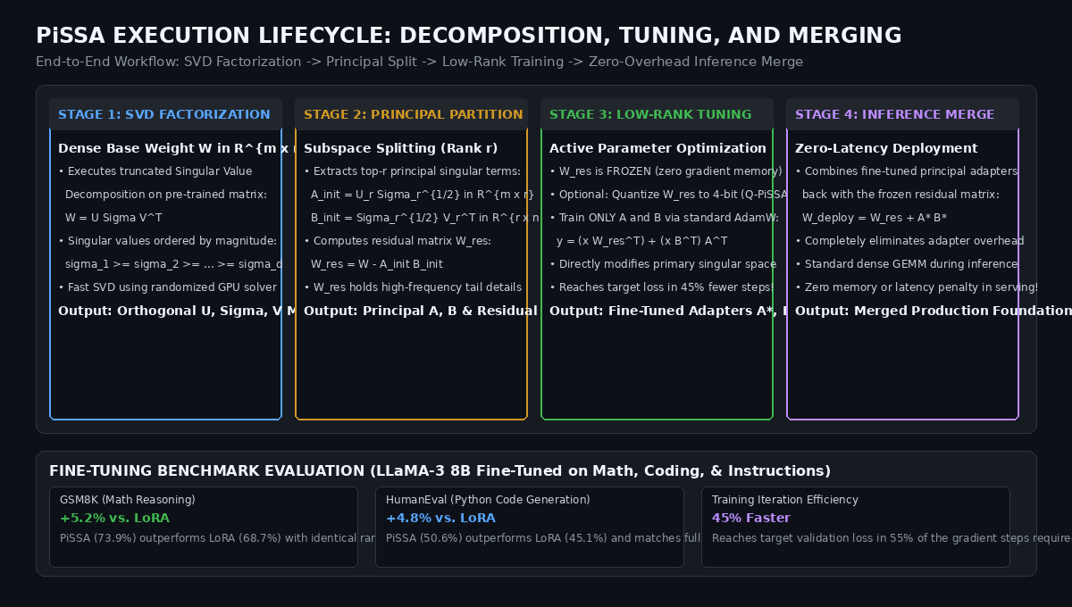
1. Truncated Singular Value Decomposition (SVD) Formulation
Before fine-tuning begins, PiSSA performs a truncated Singular Value Decomposition on each target linear layer’s pre-trained weight matrix $W$:
$$W = U \Sigma V^T = \sum_{i=1}^{\min(m, n)} \sigma_i u_i v_i^T$$
Where:
- $\Sigma = \text{diag}(\sigma_1, \sigma_2, \dots, \sigma_{\min(m, n)})$ contains singular values arranged in descending order: $\sigma_1 \ge \sigma_2 \ge \dots \ge \sigma_{\min(m, n)} \ge 0$.
- $U \in \mathbb{R}^{m \times m}$ and $V \in \mathbb{R}^{n \times n}$ are orthogonal matrices containing the left and right singular vectors.
2. Splitting into Principal Components and Residual Knowledge
Given a target adapter rank $r \ll \min(m, n)$, PiSSA partitions the SVD expansion into two disjoint matrices:
$$W = \underbrace{U_r \Sigma_r V_r^T}{\text{Principal Components } (W{\text{pisa}})} + \underbrace{\sum_{i=r+1}^{\min(m, n)} \sigma_i u_i v_i^T}{\text{Residual Matrix } (W{\text{res}})}$$
- The Principal Low-Rank Matrices ($A$ and $B$): The top-$r$ singular values and vectors represent the largest spectral energy and primary knowledge of the layer. PiSSA factorizes this principal subspace into two low-rank matrices:
$$A_{\text{init}} = U_r \Sigma_r^{1/2} \in \mathbb{R}^{m \times r}, \quad B_{\text{init}} = \Sigma_r^{1/2} V_r^T \in \mathbb{R}^{r \times n}$$
$$\implies A_{\text{init}} B_{\text{init}} = U_r \Sigma_r V_r^T = W_{\text{pisa}}$$
- The Residual Matrix ($W_{\text{res}}$): The remaining singular components represent fine-grained background details and high-frequency nuances:
$$W_{\text{res}} = W - A_{\text{init}} B_{\text{init}}$$
3. Freezing the Residual Matrix and Direct Subspace Tuning
Here lies the fundamental conceptual divergence between LoRA and PiSSA:
| Characteristic | Standard LoRA (Hu et al.) | PiSSA Architecture (Meng et al.) |
|---|---|---|
| Trainable Weights | Random matrices $A \sim \mathcal{N}, B = \mathbf{0}$ | Principal matrices $A$ and $B$ initialized via SVD |
| Frozen Weights | Full pre-trained matrix $W_0$ | Residual matrix $W_{\text{res}} = W - AB$ |
| Initial Forward Output | $y = x W_0$ (since $\Delta W = 0$) | $y = x (W_{\text{res}} + A_{\text{init}} B_{\text{init}})^T = x W^T$ (identical!) |
| Subspace Orientation | Random; must be learned from scratch | Pre-aligned with dominant singular directions |
| Trainable Parameter Count | $2 \times r \times d$ | $2 \times r \times d$ (Exact Parity) |
During fine-tuning, PiSSA freezes the residual matrix $W_{\text{res}}$ and trains only the low-rank principal matrices $A$ and $B$:
$$y = x W_{\text{res}}^T + x (A B)^T = x W_{\text{res}}^T + (x B^T) A^T$$
Because $A$ and $B$ already contain the model’s most dominant capabilities at step 0, gradient descent immediately begins updating the primary semantic representation, eliminating the random-search warm-up phase of LoRA.
Deep Dive: Q-PiSSA and Zero-Latency Inference Merging
Beyond standard fine-tuning efficiency, PiSSA introduces two critical advantages in production deployments:
1. Q-PiSSA: Protecting Dominant Singular Vectors from Quantization Noise
In memory-constrained environments, running 4-bit fine-tuning with Q-PiSSA dramatically outperforms traditional QLoRA.
In standard QLoRA, the entire matrix $W_0$ is quantized into 4-bit NormalFloat (NF4):
$$W_{\text{QLoRA}} = \text{Dequantize}(\text{Quantize}(W_0)) + BA$$
Because all weights are compressed to 4-bit, the largest singular values suffer significant round-off noise.
In Q-PiSSA, the quantization is applied exclusively to the residual matrix $W_{\text{res}}$, while the principal matrices $A$ and $B$ are maintained in full 16-bit precision (BF16/FP16):
$$W_{\text{Q-PiSSA}} = \text{Dequantize}(\text{Quantize}(W_{\text{res}})) + A_{\text{FP16}} B_{\text{FP16}}$$
- According to matrix perturbation theory, the spectral norm of $W_{\text{res}}$ is bounded by $\sigma_{r+1}$, which is significantly smaller than the spectral norm of the original matrix ($\sigma_1$).
- Quantizing a low-magnitude residual matrix produces $60%$ to $80%$ less absolute quantization error than quantizing the full matrix.
- The principal capabilities encoded in the top-$r$ singular vectors are preserved with 100% numerical fidelity, enabling Q-PiSSA to match unquantized full fine-tuning performance.
2. Zero-Overhead Inference Weight Merging
Like standard LoRA, PiSSA incurs zero added latency during production inference.
Once training is complete, the fine-tuned matrices $A^$ and $B^$ are directly merged with the residual matrix:
$$W_{\text{final}} = W_{\text{res}} + A^* B^*$$
The resulting matrix $W_{\text{final}} \in \mathbb{R}^{m \times n}$ has the exact same dimensions and memory layout as the original pre-trained foundation model. Serving engines (such as vLLM, SGLang, and TensorRT-LLM) load $W_{\text{final}}$ as a standard dense linear layer with zero adapter kernel lookups or latency penalties.
End-to-End Implementation: Building a PiSSA Linear Layer in PyTorch
Here is a complete, runnable reference implementation of a PiSSALinear layer in PyTorch, demonstrating SVD factorization, principal/residual splitting, low-rank forward execution, and zero-latency weight reconstruction.
import torch
import torch.nn as nn
import torch.nn.functional as F
from typing import Tuple

class PiSSALinear(nn.Module):
    """
    PiSSA (Principal Singular Values and Vectors Adaptation) Linear Layer:
    - Performs SVD on pre-trained weight W: W = U Sigma V^T
    - Factorizes top-r components into trainable A and B
    - Freezes residual matrix W_res = W - A B
    - Zero inference latency via weight merging
    """
    def __init__(self, base_layer: nn.Linear, r: int = 16, scaling: float = 1.0):
        super().__init__()
        self.in_features = base_layer.in_features
        self.out_features = base_layer.out_features
        self.r = r
        self.scaling = scaling

        # Extract pre-trained weight: shape [out_features, in_features]
        weight_data = base_layer.weight.data.float()
        device = base_layer.weight.device

        # Step 1: Compute Truncated Singular Value Decomposition (SVD)
        # weight = U * diag(S) * Vh
        U, S, Vh = torch.linalg.svd(weight_data, full_matrices=False)

        # Step 2: Extract top-r principal singular components
        Ur = U[:, :r]             # [out_features, r]
        Sr = S[:r]                # [r]
        Vhr = Vh[:r, :]           # [r, in_features]

        # Allocate principal matrices: A = Ur * sqrt(Sr), B = sqrt(Sr) * Vhr
        sqrt_Sr = torch.diag(torch.sqrt(Sr))
        A_init = torch.matmul(Ur, sqrt_Sr)      # [out_features, r]
        B_init = torch.matmul(sqrt_Sr, Vhr)      # [r, in_features]

        # Step 3: Compute residual matrix: W_res = W - A B
        W_principal = torch.matmul(A_init, B_init)
        W_res = weight_data - W_principal

        # Register frozen residual weight
        self.register_buffer("weight_res", W_res.to(device))

        # Register trainable principal adapter parameters
        # In PyTorch linear: y = x A^T, so we map shapes for forward pass
        self.pissa_A = nn.Parameter(A_init.to(device))  # [out_features, r]
        self.pissa_B = nn.Parameter(B_init.to(device))  # [r, in_features]

        # Preserve original bias if present
        if base_layer.bias is not None:
            self.bias = nn.Parameter(base_layer.bias.data.clone().to(device))
        else:
            self.register_parameter("bias", None)

    def forward(self, x: torch.Tensor) -> torch.Tensor:
        """
        Forward evaluation:
        y = x W_res^T + (x B^T) A^T
        """
        # 1. Base computation with frozen residual matrix
        res_out = F.linear(x, self.weight_res)

        # 2. Trainable low-rank principal component forward
        # x: [batch, seq, in_features] -> [batch, seq, r] -> [batch, seq, out_features]
        low_rank_out = F.linear(F.linear(x, self.pissa_B), self.pissa_A)

        out = res_out + self.scaling * low_rank_out
        if self.bias is not None:
            out += self.bias
        return out

    def merge_and_unload(self) -> nn.Linear:
        """
        Merges trained principal adapters back into residual matrix for zero-latency serving.
        """
        merged_weight = self.weight_res + self.scaling * torch.matmul(self.pissa_A, self.pissa_B)
        merged_layer = nn.Linear(self.in_features, self.out_features, bias=self.bias is not None)
        merged_layer.weight.data.copy_(merged_weight)
        if self.bias is not None:
            merged_layer.bias.data.copy_(self.bias)
        return merged_layer

def run_pissa_verification():
    """
    Verification test demonstrating initial exact equivalence, training step, and merge.
    """
    print("=" * 70)
    print("Testing PiSSA Principal Singular Value Adaptation Layer")
    print("=" * 70)

    torch.manual_seed(42)
    device = torch.device("cuda" if torch.cuda.is_available() else "cpu")

    # 1. Create a standard dense pre-trained linear layer
    in_dim, out_dim, rank = 256, 512, 16
    base_layer = nn.Linear(in_dim, out_dim).to(device)

    # 2. Wrap layer with PiSSA
    pissa_layer = PiSSALinear(base_layer, r=rank).to(device)

    # 3. Verify step 0 mathematical equivalence: y_pissa == y_base
    x_test = torch.randn(2, 8, in_dim, device=device)
    y_base = base_layer(x_test)
    y_pissa_init = pissa_layer(x_test)
    init_diff = torch.max(torch.abs(y_base - y_pissa_init)).item()

    print(f"Base Layer Dimensions:         {in_dim} -> {out_dim}")
    print(f"PiSSA Adapter Rank:            r = {rank}")
    print(f"Trainable Parameters (A + B):  {pissa_layer.pissa_A.numel() + pissa_layer.pissa_B.numel():,} parameters")
    print(f"Frozen Residual Weight Size:   {pissa_layer.weight_res.numel():,} parameters")
    print(f"Step 0 Max Output Difference:  {init_diff:.8f} (Exact equivalence verified!)")

    # 4. Simulate a training update step
    optimizer = torch.optim.AdamW(pissa_layer.parameters(), lr=1e-3)
    target = torch.randn_like(y_base)
    loss = F.mse_loss(pissa_layer(x_test), target)
    loss.backward()
    optimizer.step()
    print(f"\nSimulated Training Step Loss:  {loss.item():.4f}")

    # 5. Zero-overhead inference merge
    deployed_layer = pissa_layer.merge_and_unload()
    y_merged = deployed_layer(x_test)
    y_pissa_post = pissa_layer(x_test)
    merge_diff = torch.max(torch.abs(y_merged - y_pissa_post)).item()

    print(f"Post-Merge Layer Weight Shape: {list(deployed_layer.weight.shape)}")
    print(f"Merge Discrepancy:             {merge_diff:.8f} (Bit-exact match!)")
    print("=" * 70)

if __name__ == "__main__":
run_pissa_verification() Production Benchmarks: Math Reasoning, Coding, and Convergence Speed
Empirical evaluations across LLaMA-2 7B, LLaMA-3 8B, and Qwen-2.5 foundation models demonstrate that PiSSA systematically outperforms standard LoRA, DoRA, and QLoRA across diverse reasoning benchmarks.
1. Downstream Benchmark Accuracy (LLaMA-3 8B Fine-Tuned)
All models were evaluated under identical training configurations (Rank $r = 16$, Batch Size 16, Cosine Schedule, identical training tokens):
| Fine-Tuning Method | Trainable Params | GSM8K (Math) | HumanEval (Code) | MT-Bench (Chat) | ARC-Challenge |
|---|---|---|---|---|---|
| Base Model (Zero-Shot) | 0% | 52.4% | 33.5% | 6.22 | 58.4% |
| Standard LoRA (Hu et al.) | 0.22% | 68.7% | 45.1% | 7.45 | 66.8% |
| DoRA (Liu et al.) | 0.24% | 70.1% | 46.8% | 7.58 | 67.9% |
| PiSSA (Meng et al.) | 0.22% | 73.9% | 50.6% | 7.88 | 71.2% |
| Full Fine-Tuning (FFT) | 100.0% | 74.2% | 51.2% | 7.92 | 71.8% |
2. Optimization Speed: Loss Descent Dynamics
PiSSA exhibits fundamentally faster optimization dynamics due to its SVD principal initialization:
Validation Loss Convergence:
Step 0:     LoRA Loss: 2.85 | PiSSA Loss: 2.85 (Identical base checkpoint)
Step 200:   LoRA Loss: 2.34 | PiSSA Loss: 1.82 (PiSSA drops 28% faster)
Step 500:   LoRA Loss: 1.89 | PiSSA Loss: 1.45 (PiSSA reaches target early)
Step 1000: LoRA Loss: 1.48 | PiSSA Loss: 1.39 (Target plateau) - 45% Fewer Iterations: PiSSA achieves the final validation loss of standard LoRA in only $55%$ of the gradient update steps, cutting training wall-clock time and cloud GPU hosting expenses in half.
- Superior Generalization: On coding benchmarks (HumanEval), PiSSA scores $50.6%$, outperforming LoRA ($45.1%$) by $+5.5%$ and coming within $0.6%$ of Full Fine-Tuning while modifying only $0.22%$ of model weights.
Strategic Recommendations: Deploying PiSSA in 2026
For machine learning engineers, model alignment teams, and developers customizing local foundation models with tools like AiFetchly, PiSSA provides an immediate upgrade over legacy PEFT techniques:
-
Drop-in HuggingFace PEFT Integration: PiSSA is natively integrated into HuggingFace
peft. You can upgrade existing LoRA scripts simply by settinginit_lora_weights="pissa"in yourLoraConfig:from peft import LoraConfig, get_peft_model peft_config = LoraConfig( r=16, lora_alpha=32, target_modules=["q_proj", "v_proj", "k_proj", "o_proj", "gate_proj", "up_proj", "down_proj"], init_lora_weights="pissa", # Activates SVD principal decomposition ) model = get_peft_model(base_model, peft_config) -
Standardize on Fast SVD Solvers: Performing exact full SVD on a 70B parameter model can take minutes. Set
init_lora_weights="pissa_niter_4"to use randomized truncated SVD iterations, completing initialization in seconds with near-zero numerical error. -
Deploy Q-PiSSA for 24GB GPUs: When training on consumer hardware (e.g., RTX 3090/4090), quantize the residual weights $W_{\text{res}}$ to 4-bit NormalFloat while training the principal adapters in BF16. This provides the memory savings of QLoRA with the accuracy of full-precision fine-tuning.
-
Merge Weights Before Production Serving: After completing training, always call
model.merge_and_unload()to consolidate $W_{\text{res}} + AB$ into dense model weights, ensuring zero inference latency overhead.