pgvectorpostgresqlvector-databaseraghnswhybrid-searchtutorial

pgvector Guide: PostgreSQL Vector Search & HNSW Indexing

October 1, 2026

pgvector Architecture: PostgreSQL Vector Search with HNSW Graph Indexing, Halfvec Compression, Iterative Scans, and SQL Hybrid Search

The Problem: The Dual-Database Architectural Tax in Modern AI Systems

In enterprise software engineering, automated web data extraction, and intelligent desktop copilots powered by AiFetchly, foundation models rely on Retrieval-Augmented Generation (RAG) to ground their completions in proprietary knowledge. Whether indexing corporate financial statements, harvested e-commerce catalogs, or live documentation, high-dimensional vector embeddings serve as the semantic index for AI retrieval.

During the early generative AI wave, engineering teams instinctively adopted standalone, specialized vector databases (such as Pinecone, Weaviate, or Milvus). While these dedicated systems demonstrated fast nearest-neighbor benchmarks in isolated academic settings, deploying them in mission-critical production environments introduced a punishing operational penalty: the dual-database architectural tax.

The Standalone Vector Database Dilemma:
┌─────────────────────────────────────────────────────────────────┐
│ Primary Application Database (PostgreSQL)                       │
│ • User Accounts, RBAC Permissions, Billing, Documents (ACID)   │
└─────────────────────────────────────────────────────────────────┘
 │
 ├──► Dual-Write Synchronization Lag & Network Transport Latency
 ▼
┌─────────────────────────────────────────────────────────────────┐
│ Secondary Standalone Vector Database (Pinecone / Milvus)        │
│ • Floating-point Embeddings & Vector Indices (No ACID / No FK) │
└─────────────────────────────────────────────────────────────────┘
 │
 ├── ❌ Synchronization Drift: Row updated in Postgres, vector stale in Vector DB
 ├── ❌ Orphaned Embeddings: User deletes document; vector remains searchable
 ├── ❌ Dual Backup Hell: Impossible to create point-in-time consistent backups
 ├── ❌ Filtered Search Collapse: Pre-filtering drops 99% of ANN candidates
 └── ❌ Astronomical Billing: Thousands of dollars/month for redundant servers

1. The Dual-Write Synchronization Nightmare

When application state is bifurcated across two separate database engines, maintaining consistency requires distributed transactions:

Eventual Consistency Failure: A customer updates their profile or modifies a document in PostgreSQL. Before the asynchronous background queue updates the external vector store, a user query hits the vector database and retrieves stale information.
Orphaned Vectors & Data Leaks: If a database transaction rolls back in PostgreSQL due to an application exception, but the corresponding vector insertion already succeeded in the cloud vector database, the orphaned vector remains permanently indexed—creating critical data privacy and multi-tenant security vulnerabilities.
Backup & Disaster Recovery Impossibility: PostgreSQL supports continuous Write-Ahead Log (WAL) archiving and Point-in-Time Recovery (PITR). Standalone vector databases maintain completely independent snapshot schedules. Restoring from a backup inevitably results in desynchronized state where vectors reference deleted database primary keys.

2. The Filtered Search Collapse (The Over-Filtering Trap)

In real-world enterprise RAG, vector queries are virtually never unbounded global searches. They are strictly scoped by relational metadata:

-- Real-world enterprise query requirement:
SELECT * FROM document_chunks
WHERE organization_id = 'org_9821'
  AND access_tier = 'confidential'
  AND created_at >= '2026-01-01'
ORDER BY embedding <=> query_vector
LIMIT 5;

Standalone vector databases attempt to solve this via pre-filtering or post-filtering:

Post-Filtering: The vector engine retrieves the top 100 nearest neighbors globally, and then applies the metadata filter. If only 2 of those 100 vectors belong to org_9821, the query returns an incomplete result set (2 items instead of the requested 5) or empty results entirely.
Pre-Filtering: The engine filters vectors first, but because the vectors are decoupled from the relational B-Tree indices of PostgreSQL, it must traverse unoptimized document ID sets, destroying sub-millisecond retrieval latency.

3. The Infrastructure Cost & Security Overhead

Maintaining dedicated vector clusters introduces severe financial and regulatory burdens:

Cloud vector providers charge thousands of dollars per month for managed compute and RAM.
Engineering teams must manage duplicate access control policies, TLS configurations, compliance certifications (SOC 2, HIPAA, GDPR), and monitoring alerts across two disparate systems.

The Solution: pgvector’s Native In-Database Vector Intelligence

To eliminate the dual-database tax, the open-source community created pgvector.

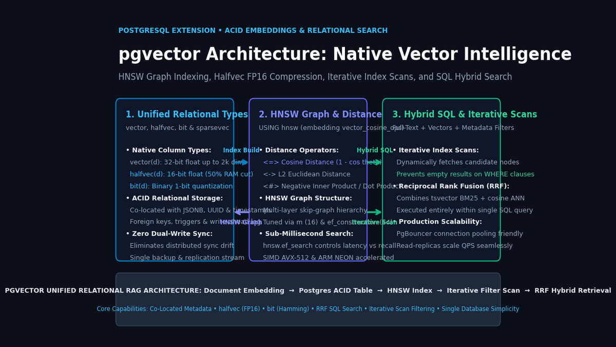
pgvector is an open-source extension written in C that transforms PostgreSQL into a high-performance vector database. By introducing native vector data types, SIMD-accelerated distance metrics, and state-of-the-art Hierarchical Navigable Small World (HNSW) graph indexing directly inside Postgres, pgvector allows software engineers to store embeddings alongside relational tables, execute hybrid queries in standard SQL, and enforce full ACID consistency.

The Unified pgvector Architecture:
┌─────────────────────────────────────────────────────────────────┐
│ Client Request (Application / aiFetchly Data Pipeline)          │
└─────────────────────────────────────────────────────────────────┘
 │
 ▼ (Single TCP Connection / PgBouncer Pool)
┌─────────────────────────────────────────────────────────────────┐
│ PostgreSQL Engine with pgvector Extension                       │
│                                                                 │
│ ┌─────────────────────────────────────────────────────────────┐ │
│ │ Unified ACID Relational Table: document_chunks               │ │
│ │ • id (UUID, Primary Key)                                    │ │
│ │ • organization_id (UUID, B-Tree Index, Foreign Key)         │ │
│ │ • content (TEXT, tsvector Full-Text Search Index)           │ │
│ │ • metadata (JSONB, GIN Index)                               │ │
│ │ • embedding (halfvec(1536), HNSW Cosine Index)              │ │
│ └─────────────────────────────────────────────────────────────┘ │
│                                                                 │
│ • Single Transactional Log (WAL): Zero synchronization drift   │
│ • Single Unified Backup: Point-in-time recovery for everything │
│ • Hardware Acceleration: AVX-512, AVX2 & ARM NEON SIMD kernels  │
│ • Query Optimizer: Combines B-Tree, GIN, and HNSW dynamically │
└─────────────────────────────────────────────────────────────────┘

The Core Architectural Pillars of pgvector

Relational Co-Location: High-dimensional embeddings are stored as standard table columns alongside primary keys, foreign keys, timestamps, and JSONB payloads. An UPDATE or DELETE on a table row atomically modifies both relational data and vector indices in a single ACID transaction.
HNSW Graph Indexing: Implements multi-layer Hierarchical Navigable Small World graphs directly within Postgres buffer pools, delivering sub-millisecond Approximate Nearest Neighbor (ANN) search with 99%+ recall.
Half-Precision & Binary Quantization: Native support for 16-bit floats (halfvec) cuts index memory footprint in half with zero loss in retrieval precision, while 1-bit vectors (bit) reduce memory consumption by up to 95% using bit-level Hamming distance.
Iterative Index Scans: Solves the filtered search trap by dynamically traversing the HNSW graph until the target number of rows matching the relational WHERE clause are discovered.
Unified SQL Hybrid Search: Enables combining dense vector similarity with Postgres full-text lexical search (tsvector / BM25) using Reciprocal Rank Fusion (RRF) in a single, elegant SQL query.

Comparing Vector Storage Paradigms

The table below contrasts pgvector against standalone cloud vector databases and un-indexed SQL search:

Vector Database Architectural Comparison:
┌───────────────────────────┬───────────────────────────────┬───────────────────────────────┬───────────────────────────────┐
│ Architectural Dimension   │ Naive SQL (Cosine in Postgres)│ Standalone Vector DB (Cloud)  │ PostgreSQL with pgvector      │
├───────────────────────────┼───────────────────────────────┼───────────────────────────────┼───────────────────────────────┤
│ Transactional Consistency │ Full ACID                     │ ❌ Eventual consistency / None│ Full ACID (Atomic writes)     │
│ Query Latency (1M vectors)│ 1,500ms–5,000ms (Sequential)  │ 2ms–15ms (Dedicated ANN)      │ 2ms–8ms (HNSW Graph ANN)      │
│ Memory Optimization       │ None (Unindexed raw arrays)   │ Proprietary quantization      │ halfvec (FP16), bit (1-bit)   │
│ Relational Joins & Filters│ Native SQL joins              │ ❌ Brittle post/pre-filtering │ Native iterative index scans  │
│ Hybrid Full-Text Search   │ Requires custom glue code     │ Separate keyword index service│ Native SQL tsvector + RRF     │
│ Backup & Recovery         │ Standard pg_dump / pg_basebackup│ Disjointed independent snapshots│ Unified WAL Point-In-Time (PITR)│
│ Infrastructure Overhead   │ Zero extra servers            │ High (Separate cluster & bills)│ Zero extra servers            │
└───────────────────────────┴───────────────────────────────┴───────────────────────────────┴───────────────────────────────┘

Deep Dive into pgvector Primitives & Index Structures

pgvector integrates into the PostgreSQL type system and query planner through specialized column types, hardware-accelerated distance operators, and sophisticated index traversal routines.

pgvector Core Primitives:
pgvector Engine
 ├──► 1. Column Types: vector (fp32), halfvec (fp16), bit (1-bit), sparsevec
 ├──► 2. Distance Operators: <=> (Cosine), <-> (Euclidean L2), <#> (Inner Prod)
 ├──► 3. Index Types: HNSW (Graph-based, fast), IVFFlat (Cluster-based, small)
 ├──► 4. Iterative Index Scans: hnsw.iterative_scan for relational WHERE clauses
 └──► 5. Hybrid Search: SQL CTE combining tsvector BM25 and vector embeddings

1. Native Data Types: `vector`, `halfvec`, and `bit`

pgvector provides four distinct representations tailored to different accuracy and memory profiles:

vector(d): Standard 32-bit single-precision floating-point format supporting up to 2,000 dimensions (or up to 16,000 without an index). Ideal for maximum precision.
halfvec(d): 16-bit half-precision floating-point format (IEEE 754 float16) supporting up to 4,000 dimensions. It stores embeddings using 50% less RAM and disk space while maintaining 99.8%+ identical recall compared to float32.
bit(d): 1-bit binary vector format supporting up to 64,000 dimensions. When paired with binary quantization embeddings, bit compresses vectors by 32x (96% memory reduction) and computes distances via single-cycle CPU hardware Hamming instructions (POPCNT).
sparsevec(d): Sparse vector representation storing up to 1,000 non-zero elements across high-dimensional token vocabularies (e.g., for learned sparse models like SPLADE or BM25 term weights).

2. Distance Operators and SIMD Execution

Distance calculations in pgvector are executed via custom C routines compiled with vectorization flags (-mavx512f, -mavx2, -mfma on x86, or NEON on ARM):

Cosine Distance (<=>): Computes $1 - \frac{u \cdot v}{|u|_2 |v|_2}$. Standard metric for text embeddings (OpenAI, Voyage, Cohere).
Euclidean L2 Distance (<->): Computes $\sqrt{\sum (u_i - v_i)^2}$. Preferred for image embeddings and clustering.
Negative Inner Product (<#>): Computes $-(u \cdot v)$. When vectors are unit-normalized, inner product is mathematically identical to cosine similarity but skips square-root normalization, yielding faster query throughput.
Hamming Distance (<~>): Computes bit-level difference counts for binary quantized vectors.

3. HNSW vs. IVFFlat: Selecting the Optimal Index

Postgres supports two primary index structures for vector columns:

HNSW vs. IVFFlat Architectural Structure:
HNSW (Hierarchical Navigable Small World)   IVFFlat (Inverted File Flat)
Layer 2: [Entry Point] ──► [Node A]         Centroid 1 ──► [Vec 1, Vec 2, Vec 3]
            │                 │             Centroid 2 ──► [Vec 4, Vec 5, Vec 6]
Layer 1: [Node B] ──► [Node C] ──► [Node D] Centroid 3 ──► [Vec 7, Vec 8, Vec 9]
            │           │           │
Layer 0: [Dense Graph with all Vectors]     Query: Scans closest lists centroids
Search: Sub-millisecond skip traversal      Search: Linear scan within assigned clusters
Build: Compute-intensive, high RAM          Build: Fast build, low RAM, requires warm data

HNSW (Recommended for Production):
- Builds a multi-layer geometric graph structure similar to a probabilistic skip list.
- Queries enter at top sparse layers and traverse rapidly toward local neighborhoods before descending to the dense base layer.
- Controlled by two parameters: m (maximum connections per node, default 16) and ef_construction (candidate search depth during build, default 64).
- Runtime speed vs. recall is dynamically tuned per session via SET hnsw.ef_search = 100;.
- Verdict: Far superior query latency and recall; handles dynamic inserts without index degradation.
IVFFlat:
- Partitions vector space into Voronoi cells using k-means clustering.
- Requires training on an existing dataset to calculate cluster centroids (lists = rows / 1000).
- Verdict: Slower query latency and sensitive to data distribution shift, but builds quickly and uses minimal RAM.

4. Solving the Filtered Search Dilemma: Iterative Index Scans

Historically, executing WHERE category = 'finance' ORDER BY embedding <=> query LIMIT 10 on an HNSW index caused failures if finance represented a small fraction of the database:

The HNSW index would return its nearest 40 neighbors; if none belonged to finance, Postgres fell back to a catastrophic sequential table scan.
In modern pgvector, Iterative Index Scans resolve this:

SET hnsw.iterative_scan = 'relaxed';

When enabled, pgvector dynamically continues searching further out along the HNSW graph until it discovers the requested LIMIT of valid rows that satisfy the relational predicate, guaranteeing fast, complete results even on highly selective filters.

Hands-On Implementation: Building a Production Vector RAG Store

Let’s implement a complete enterprise RAG storage and retrieval engine in PostgreSQL with pgvector. We will configure halfvec compression, build an HNSW index, and execute hybrid search combining dense vectors with full-text search via Reciprocal Rank Fusion (RRF).

1. Enabling the Extension & Creating the Schema

Connect to your PostgreSQL database and enable vector:

-- 1. Enable the pgvector extension
CREATE EXTENSION IF NOT EXISTS vector;

-- 2. Create the unified document chunk table
CREATE TABLE document_chunks (
    id UUID PRIMARY KEY DEFAULT gen_random_uuid(),
    document_id UUID NOT NULL,
    organization_id UUID NOT NULL,
    title TEXT NOT NULL,
    content TEXT NOT NULL,
    metadata JSONB DEFAULT '{}'::jsonb,

    -- Full-Text Search tsvector column for lexical search
    tsv_content tsvector GENERATED ALWAYS AS (to_tsvector('english', title || ' ' || content)) STORED,

    -- 16-bit half-precision vector for 50% memory savings (1536 dimensions)
    embedding halfvec(1536) NOT NULL,

    created_at TIMESTAMPTZ DEFAULT clock_timestamp()
);

-- 3. Create relational B-Tree and GIN indexes
CREATE INDEX idx_chunks_org_id ON document_chunks (organization_id);
CREATE INDEX idx_chunks_tsv ON document_chunks USING gin(tsv_content);
CREATE INDEX idx_chunks_metadata ON document_chunks USING gin(metadata);

2. Building the Memory-Optimized HNSW Index

Before building the index on large datasets, allocate sufficient maintenance memory:

-- Allocate 2GB memory for fast index construction
SET maintenance_work_mem = '2GB';
SET max_parallel_maintenance_workers = 4;

-- Build HNSW index using cosine distance operator class
CREATE INDEX idx_chunks_hnsw_embedding ON document_chunks
USING hnsw (embedding halfvec_cosine_ops)
WITH (m = 16, ef_construction = 128);

3. Inserting Sample Vectors in Python

Using psycopg and pgvector in Python:

import psycopg
from pgvector.psycopg import register_vector
import numpy as np

# Connect to Postgres
conn = psycopg.connect("postgresql://postgres:password@localhost:5432/rag_db")
register_vector(conn)

cursor = conn.cursor()

# Generate dummy 1536-dim embedding normalized to unit sphere
raw_vector = np.random.randn(1536).astype(np.float16)
raw_vector = raw_vector / np.linalg.norm(raw_vector)

cursor.execute("""
    INSERT INTO document_chunks (
        document_id, organization_id, title, content, embedding
    ) VALUES (
        gen_random_uuid(), gen_random_uuid(), %s, %s, %s
    );
""", (
    "Q3 Financial Performance Report",
    "Nvidia reported data center revenue growth of 112% year-over-year in Q3 FY25.",
    raw_vector
))

conn.commit()
print("Successfully inserted document with halfvec embedding!")

4. Executing Single-Query Hybrid Search (RRF) in SQL

Combine dense vector semantic similarity with full-text keyword search using Reciprocal Rank Fusion (RRF) directly in SQL:

-- Set search depth for HNSW index traversal
SET hnsw.ef_search = 100;
SET hnsw.iterative_scan = 'relaxed';

WITH semantic_search AS (
    -- Stage 1: Dense Vector Retrieval (Top 50)
    SELECT
        id,
        ROW_NUMBER() OVER (ORDER BY embedding <=> '[0.012, -0.043, ...]'::halfvec) AS rank
    FROM document_chunks
    WHERE organization_id = 'c7a8b412-421b-4f5a-9321-7218ef892112'
    ORDER BY embedding <=> '[0.012, -0.043, ...]'::halfvec
    LIMIT 50
),
keyword_search AS (
    -- Stage 2: Lexical Full-Text Search via BM25 / tsvector (Top 50)
    SELECT
        id,
        ROW_NUMBER() OVER (ORDER BY ts_rank_cd(tsv_content, plainto_tsquery('english', 'Nvidia revenue growth')) DESC) AS rank
    FROM document_chunks
    WHERE organization_id = 'c7a8b412-421b-4f5a-9321-7218ef892112'
      AND tsv_content @@ plainto_tsquery('english', 'Nvidia revenue growth')
    LIMIT 50
)
-- Stage 3: Reciprocal Rank Fusion (RRF with k=60)
SELECT
    d.id,
    d.title,
    d.content,
    COALESCE(1.0 / (60 + s.rank), 0.0) + COALESCE(1.0 / (60 + k.rank), 0.0) AS rrf_score
FROM document_chunks d
LEFT JOIN semantic_search s ON d.id = s.id
LEFT JOIN keyword_search k ON d.id = k.id
WHERE s.id IS NOT NULL OR k.id IS NOT NULL
ORDER BY rrf_score DESC
LIMIT 10;

Production Architecture & Performance Tuning for aiFetchly

Integrating pgvector into high-throughput data extraction, web scraping, and desktop intelligence systems like AiFetchly requires strict hardware alignment and configuration tuning.

aiFetchly Enterprise Data Ingestion & Storage Architecture:
┌─────────────────────────────────────────────────────────────────┐
│ aiFetchly Desktop Application & Web Extraction Engine           │
│ • Parallel document scrapers, PDF parsers, and API harvesters   │
└─────────────────────────────────────────────────────────────────┘
 │
 ▼ (Batch Embeddings Stream)
┌─────────────────────────────────────────────────────────────────┐
│ PgBouncer Connection Pooler (Transaction Mode)                  │
│ • Absorbs hundreds of client agent connections                  │
│ • Manages ephemeral worker transactions without backend stalls  │
└─────────────────────────────────────────────────────────────────┘
 │
 ▼
┌─────────────────────────────────────────────────────────────────┐
│ Primary PostgreSQL Node (Writes & WAL Generation)               │
│ • Ingests structured JSONB + halfvec embeddings atomically      │
│ • Background autovacuum optimizes HNSW graph and B-Trees        │
└─────────────────────────────────────────────────────────────────┘
 │
 ├──► WAL Streaming Replication (Near Zero Latency)
 ▼
┌─────────────────────────────────────────────────────────────────┐
│ Read Replica Pool (High-Concurrency Vector Queries)             │
│ • HNSW indexes locked in RAM (shared_buffers + OS Cache)        │
│ • Dispatches parallel hybrid RRF queries to downstream LLMs     │
└─────────────────────────────────────────────────────────────────┘

1. Memory Sizing: The HNSW RAM Formula

For fast query execution, HNSW graph structures must reside entirely in memory (either in PostgreSQL shared_buffers or the operating system’s filesystem cache):

Float32 Vector Index Size: $$\text{RAM per Vector} \approx (\text{Dimensions} \times 4 \text{ bytes}) + (M \times 2 \times 8 \text{ bytes})$$ For 1,000,000 vectors of 1,536 dimensions with $M=16$: $$\text{Index Size} \approx 6.14\text{ GB (Vectors)} + 0.25\text{ GB (Graph)} \approx 6.4\text{ GB}$$
Halfvec (FP16) Vector Index Size: $$\text{RAM per Vector} \approx (\text{Dimensions} \times 2 \text{ bytes}) + (M \times 2 \times 8 \text{ bytes})$$ $$\text{Index Size} \approx 3.07\text{ GB (Vectors)} + 0.25\text{ GB (Graph)} \approx 3.3\text{ GB (50% Reduction!)}$$
Always allocate at least 1.2x the calculated index size to shared_buffers plus available host RAM to prevent high-latency random NVMe disk seeks during graph traversal.

2. PgBouncer Connection Pooling in Transaction Mode

When serving thousands of desktop agents or microservices, connect through PgBouncer:

Use pool_mode = transaction to minimize server backend process overhead.
Because parameters like hnsw.ef_search are session-level variables, set them at the user or database level rather than per-connection:

ALTER DATABASE rag_db SET hnsw.ef_search = 100;
ALTER DATABASE rag_db SET hnsw.iterative_scan = 'relaxed';

3. Correlating Database Embeddings with Multi-Agent Observability

In production pipelines:

Co-locate chunk vector IDs with execution spans tracked in Langfuse or DeepEval.
When an agent retrieves a low-relevance chunk, log the document_chunks.id directly into your evaluation traces.
Use continuous evaluation to benchmark whether increasing m or updating the embedding model improves RAG faithfulness without altering backend database schemas.

Summary: The Power of Database Simplicity in AI Engineering

The trajectory of production software engineering consistently favors consolidation over architectural sprawl. Just as PostgreSQL previously absorbed JSON document storage (supplanting ad-hoc document databases) and spatial data (via PostGIS), pgvector now renders standalone vector databases redundant for the vast majority of enterprise use cases.

By combining sub-millisecond HNSW graph indexing, native halfvec memory compression, iterative index scans for complex relational predicates, and SQL-native hybrid search, pgvector allows engineering teams to build robust, scalable AI applications on top of the world’s most battle-tested relational database. For high-volume web scrapers, automated document extractors, and desktop AI copilots engineered with AiFetchly, pgvector delivers uncompromised vector performance with rock-solid ACID reliability.