NVIDIA Minitron Guide: Fast LLM Pruning & Distillation
The Problem: The Pretraining Compute Wall of Small Language Models
In modern enterprise automation, developer desktop copilots, and autonomous scraping assistants like AiFetchly, deploying Small Language Models (SLMs)—ranging between 2 billion and 8 billion parameters—has shifted from a niche edge experiment to an architectural imperative. Running high-reasoning models locally on commodity workstations eliminates recurrent cloud API token costs, protects proprietary data privacy, and guarantees sub-10ms operational latency.
However, creating high-performing compact models has historically collided with a punishing economic barrier: the pretraining compute wall.
The Small Language Model Pretraining Dilemma:
Option A: Pretrain Compact 4B Model From Scratch
  ├── Corpus: 3 to 10 Trillion high-quality tokens (FineWeb, DCLM)
  ├── Compute: Tens of thousands of H100 GPU hours ($1M - $5M expenditure)
  └── Outcome: Prohibitive capital costs for 99% of enterprise engineering teams

Option B: Post-Training Quantization (INT4 / FP4 on 8B-15B checkpoints)
  ├── Weight Footprint: Halved in VRAM, but active FLOPs remain unchanged
  ├── Attention Heads: Fixed head count retains high KV cache memory
  └── Outcome: Still exceeds memory budgets on low-power 16GB RAM developer laptops

Option C: Traditional Unstructured / 2:4 Sparse Pruning
  ├── Hardware Friction: Requires custom CUDA sparse kernels or Blackwell hardware
└── Outcome: Zero acceleration on consumer CPUs, Apple Silicon Metal, or vLLM engines 1. The Multi-Trillion Token Tax of Pretraining from Scratch
When foundation model labs train state-of-the-art small language models—such as Llama-3.2 (1B and 3B), SmolLM2 (1.7B), or Qwen2.5 (1.5B and 3B)—they compensate for smaller parameter capacity by training on massive token volumes:
- Llama-3.2 3B was pre-trained on approximately 9 trillion tokens.
- Processing 9 trillion tokens through even a 3B-parameter transformer requires hundreds of thousands of accelerator hours, running continuously on multi-million-dollar supercomputing clusters.
- For enterprise organizations wishing to build a specialized, sovereign, on-device SLM tailored to proprietary codebases or document-extraction schemas, pretraining from scratch is economically unviable.
2. The Limitations of Quantization and Classical Weight Pruning
To shrink existing open models (like Llama-3.1 8B or Mistral-NeMo 12B), teams commonly turn to post-training quantization (AWQ, GPTQ, GGUF):
- While 4-bit quantization reduces disk footprint and weight memory bandwidth, the computational graph remains identical: the model must still evaluate 32 layers, 32 attention heads, and wide MLP matrices.
- Furthermore, classical unstructured pruning (zeroing out individual matrix weights) creates non-contiguous memory access patterns that run slower on standard tensor libraries than dense baselines.
- While semi-structured pruning (such as NVIDIA 2:4 sparsity via Wanda) accelerates matrix multiplication on Ampere and Hopper GPUs, it provides zero speedup on consumer Apple Silicon unified memory or CPU inference backends.
Production desktop workflows require a method to derive physically smaller, standard dense models that run out-of-the-box on any hardware without requiring multi-million-dollar pretraining budgets.
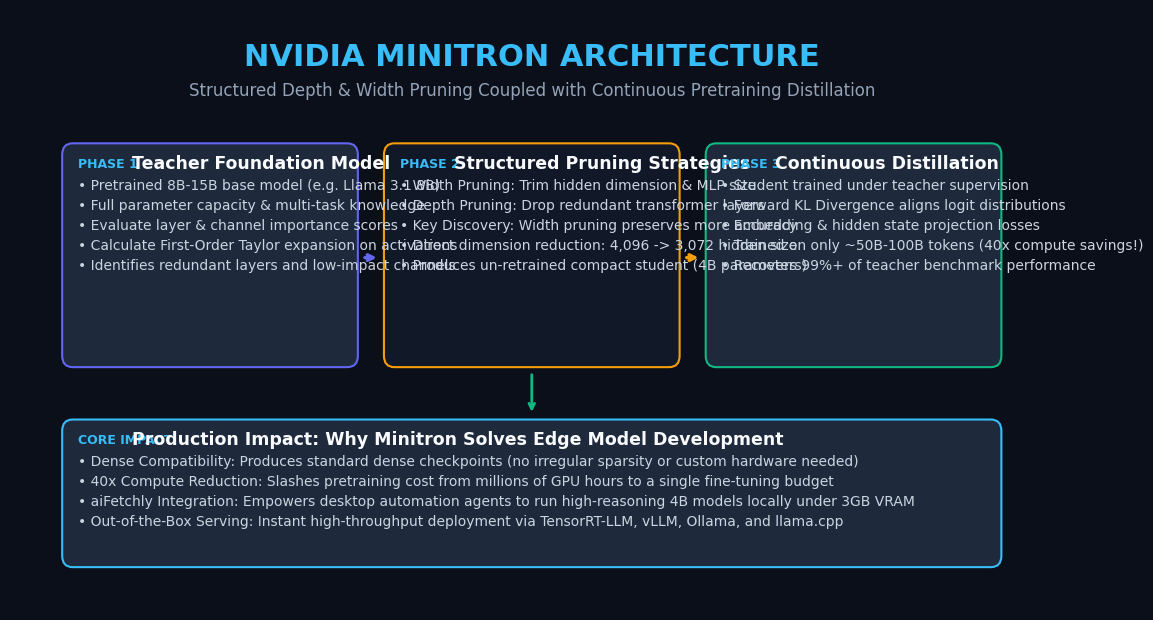
The Solution: The NVIDIA Minitron Pruning and Distillation Framework
Introduced by NVIDIA Research (Dan Zhao, Saurav Muralidharan, et al.), Minitron provides a systematic, mathematically principled methodology for compressing large pretrained foundation models into compact, dense Small Language Models using up to 40x less training compute than training from scratch.
Rather than initializing random weights and training across 10 trillion tokens, Minitron leverages two coupled techniques:
- Targeted Structured Pruning: Evaluating weight and activation saliency to physically delete entire transformer layers (depth pruning) or trim hidden state dimensions and MLP widths (width pruning).
- Continuous Distillation Retraining: Using the original, unpruned teacher model to supervise the student over a modest calibration dataset (typically 50 to 100 billion tokens), recovering degraded accuracy in a fraction of the time.
The End-to-End Minitron Pipeline:
┌────────────────────────────────────────────────────────┐
│ Pretrained Teacher Model (e.g. Llama-3.1-8B Base)      │
│ Hidden: 4,096 | Layers: 32 | FFN Intermediate: 14,336   │
└────────────────────────────────────────────────────────┘
                           │
                           ▼
 [Step 1: Calibration & Saliency Analysis (Tiny Corpus)]
 • Compute First-Order Taylor Expansion on Activations
 • Score layer redundancy vs. hidden dimension saliency
                           │
                           ▼
 [Step 2: Structured Pruning (Width vs. Depth)]
 • Width-Prune: d_model 4,096 ──► 3,072 | FFN 14,336 ──► 9,216
 • Physical slice: Eliminates parameters, creates dense student
                           │
                           ▼
 ┌────────────────────────────────────────────────────────┐
│ Dense Student Model Checkpoint (Minitron 4B)           │
│ (Un-retrained: Perplexity temporarily spikes)          │
└────────────────────────────────────────────────────────┘
                           │
                           ▼
 [Step 3: Continuous Knowledge Distillation Retraining]
 • Forward KL Divergence Loss: Aligns student & teacher logits
 • Embedding Projection Loss: Aligns input token representations
 • Intermediate Hidden State Loss: Matches layer representations
 • Dataset: Only 50B - 94B tokens (~1% of pretraining compute!)
                           │
                           ▼
 ┌────────────────────────────────────────────────────────┐
│ Production-Ready Llama-3.1-Minitron-4B                 │
│ • Matches scratch-trained 4B models on MMLU & GSM8K    │
│ • Standard dense weights: 100% compatible with vLLM,   │
│   Ollama, llama.cpp, and TensorRT-LLM                  │
└────────────────────────────────────────────────────────┘ The Three Core Innovations of Minitron
1. True Dense Architecture Output
Unlike sparsity techniques that mask weights to zero while retaining tensor dimensions, Minitron executes physical matrix resizing:
- A weight matrix $W \in \mathbb{R}^{4096 \times 14336}$ is physically sliced into $W_{\text{pruned}} \in \mathbb{R}^{3072 \times 9216}$.
- The resulting student model is a completely standard dense transformer. It requires no specialized sparse kernels, custom CUDA compilers, or proprietary runtimes.
- It deploys seamlessly across Ollama, vLLM, TensorRT-LLM, Hugging Face Transformers, and llama.cpp.
2. The Width vs. Depth Empirical Discovery
One of the most consequential findings from the Minitron research paper is the performance divergence between pruning dimensions:
- Depth Pruning (Dropping Layers): Removing layers significantly alters the model’s sequential computational depth and receptive field, leading to severe degradation on multi-step reasoning, mathematical derivation, and coding benchmarks.
- Width Pruning (Trimming Dimensions): Trimming the embedding dimension $d_{model}$ and intermediate feed-forward dimension $d_{ffn}$ while preserving all 32 layers retains dramatically higher representational capacity.
- NVIDIA demonstrated that Width-Pruned Minitron models consistently outperform Depth-Pruned variants at identical parameter counts.
3. 40x Pretraining Compute Reduction
By inheriting pretrained weights from an 8B teacher and transferring knowledge via distillation:
Llama-3.1-Minitron-4Bwas retrained on only 94 billion tokens of public data.- Compared to training a 4B model from scratch on 4 trillion tokens, Minitron achieved identical or superior benchmark scores using less than 2.5% of the computational FLOPs.
Deep Dive: Saliency Scoring and Distillation Losses
The mathematical foundation of Minitron rests on two core mechanisms: how to choose which channels to slice, and how to transfer knowledge from the teacher during distillation.
1. Estimating Parameter Importance via Taylor Expansion
To decide which rows and columns of attention heads and MLP matrices to prune, Minitron avoids naive magnitude pruning (which drops weights based strictly on $|W|$). Instead, it evaluates activation-aware saliency using a first-order Taylor expansion over a small calibration dataset:
$$\mathcal{I}{W{i,j}} = \left| \frac{\partial \mathcal{L}}{\partial W_{i,j}} \cdot W_{i,j} \right|$$
Where:
- $\mathcal{L}$ is the cross-entropy language modeling loss computed over a small calibration corpus (e.g., 1,024 sequences from the pretraining distribution).
- $\frac{\partial \mathcal{L}}{\partial W_{i,j}}$ represents the first-order gradient of the loss with respect to weight parameter $W_{i,j}$.
- Multiplying the gradient by the weight magnitude estimates the first-order change in loss if that weight were set to zero.
To prune a full hidden channel $k$ across all layers: $$\mathcal{S}k = \sum{l=1}^{L} \sum_{i} \mathcal{I}{W^{(l)}{i,k}}$$
The channels with the lowest cumulative saliency scores $\mathcal{S}_k$ are pruned, ensuring that high-magnitude weights interacting with rare activation outliers are strictly protected.
Width Pruning in SwiGLU Feed-Forward Networks:
Teacher MLP Layer:
  Gate Projection:  W_gate  [Hidden: 4,096 ──► FFN: 14,336]
  Up Projection:    W_up    [Hidden: 4,096 ──► FFN: 14,336]
  Down Projection:  W_down  [FFN: 14,336  ──► Hidden: 4,096]

Saliency Sorting & Physical Slicing:
  1. Rank 14,336 intermediate neurons by cumulative Taylor importance
  2. Retain top 9,216 neurons; discard bottom 5,120 neurons
  3. Rank 4,096 hidden channels; retain top 3,072 channels

Resulting Minitron-4B MLP Layer:
  Gate Projection:  W_gate' [Hidden: 3,072 ──► FFN: 9,216]
  Up Projection:    W_up'   [Hidden: 3,072 ──► FFN: 9,216]
Down Projection: W_down' [FFN: 9,216 ──► Hidden: 3,072] 2. Multi-Objective Distillation Loss Formulation
Immediately after physical pruning, the student model suffers a temporary loss in coherence because interconnected dimensions have been excised. To rapidly heal the model, continuous distillation is conducted using a compound loss function:
$$\mathcal{L}{\text{total}} = \alpha \mathcal{L}{\text{LM}} + \beta \mathcal{L}{\text{KD_logits}} + \gamma \mathcal{L}{\text{hidden}} + \delta \mathcal{L}_{\text{embed}}$$
1. Hard Language Modeling Loss ($\mathcal{L}_{\text{LM}}$)
Standard autoregressive next-token cross-entropy on ground-truth training tokens: $$\mathcal{L}{\text{LM}} = - \sum{t=1}^T \log P_{\text{student}}(x_t \mid x_{<t})$$
2. Forward Logit Distillation ($\mathcal{L}_{\text{KD_logits}}$)
Kullback-Leibler (KL) divergence between the teacher’s softened output distribution and the student’s output distribution: $$\mathcal{L}{\text{KD_logits}} = \tau^2 \sum{t=1}^T D_{\text{KL}}\left( \text{Softmax}\left(\frac{\mathbf{z}_t^{\text{teacher}}}{\tau}\right) \parallel \text{Softmax}\left(\frac{\mathbf{z}_t^{\text{student}}}{\tau}\right) \right)$$ Where $\tau$ is the distillation temperature (typically set to $1.0$ or $1.5$). Forward KL penalizes the student heavily when it assigns low probability to tokens the teacher considers plausible.
3. Intermediate Hidden State Projection ($\mathcal{L}_{\text{hidden}}$)
Because the student’s hidden dimension $d_{\text{student}} = 3072$ differs from the teacher’s $d_{\text{teacher}} = 4096$, the student’s hidden states cannot be directly subtracted. Minitron introduces a learnable linear projection matrix $W_{\text{proj}} \in \mathbb{R}^{3072 \times 4096}$: $$\mathcal{L}{\text{hidden}} = \sum{l \in \text{sampled}} \left| \mathbf{h}{l}^{\text{teacher}} - W{\text{proj}} \mathbf{h}_{l}^{\text{student}} \right|_2^2$$ This guides the student to mirror intermediate semantic reasoning representations rather than merely mimicking final logits.
Architectural Comparison: Minitron vs. Alternative Compression Paradigms
To understand where Minitron fits in the modern AI optimization ecosystem, the table below compares it against standard training, Parameter-Efficient Fine-Tuning (LoRA), and weight-activation pruning (Wanda):
| Dimension | Pretraining from Scratch (Llama 3.2 3B) | LoRA Fine-Tuning (PEFT) | Unstructured / 2:4 Sparsity (Wanda) | NVIDIA Minitron (Structured + KD) |
|---|---|---|---|---|
| Model Size Reduction | Native compact size | 0% (Base model unchanged) | 50% Weights (Sparsity mask) | Direct Physical Reduction (e.g. 8B ──► 4B) |
| Compute Required | Massive (3T - 10T tokens) | Minimal (Task-specific dataset) | Zero Retraining (<1 GPU hr) | Low (50B - 100B tokens, ~2.5% of pretraining) |
| Hardware Compatibility | Universal Dense | Universal Dense | Requires Sparse Tensor Cores | Universal Dense (CPU, Metal, GPU, Edge) |
| KV Cache Footprint | Fixed by architecture | Unchanged (8B footprint) | Unchanged (8B head dimensions) | Slashed (Fewer heads & narrower KV vectors) |
| Knowledge Transfer | Learned from raw internet | Constrained to adapter rank | Zero transfer (Pruning only) | Full Teacher Knowledge Distillation |
| Downstream Serving | Standard vLLM / Ollama | Merged weights in vLLM | Custom sparse kernels | Standard vLLM, TensorRT-LLM, Ollama |
| Reasoning Retention | Baseline for parameter size | Preserves base reasoning | Moderate degradation at 50% | 95% - 99% of 8B Teacher Performance |
Practical Implementation: Building a Minitron-Style Pruning & Distillation Pipeline
Let us implement a complete, reproducible Python demonstration using PyTorch and Hugging Face Transformers. In this tutorial, we will:
- Load a multi-head transformer layer.
- Calculate channel importance based on activation norms and gradients.
- Physically slice the weight matrices to create a compact student.
- Execute knowledge distillation using forward KL divergence and projection losses.
Step 1: Environment Setup
pip install torch transformers datasets accelerate Step 2: Implement Saliency Trimming and Layer Slicing
Save the following code as minitron_prune.py:
import torch
import torch.nn as nn
import torch.nn.functional as F
from typing import Tuple

class MinitronLinearPruner:
    """
    Simulates structured width pruning on a linear projection layer
    by estimating channel saliency via activation norms and weight magnitudes.
    """
    @staticmethod
    def compute_channel_saliency(layer: nn.Linear, input_activations: torch.Tensor) -> torch.Tensor:
        """
        Computes first-order importance score for each input channel:
        Saliency = Mean(|Activation|) * Mean(|Weight|)
        """
        # input_activations: [batch_size, seq_len, in_features]
        act_importance = input_activations.abs().mean(dim=(0, 1)) # [in_features]
        weight_importance = layer.weight.abs().mean(dim=0)        # [in_features]

        # Combined Taylor-inspired saliency
        saliency = act_importance * weight_importance
        return saliency

    @classmethod
    def prune_linear_layer(
        cls,
        original_layer: nn.Linear,
        target_in_features: int,
        target_out_features: int,
        saliency_scores: torch.Tensor
    ) -> nn.Linear:
        """
        Physically slices the weight tensor, discarding low-saliency channels.
        """
        # Select top-k input channels
        _, top_in_indices = torch.topk(saliency_scores, target_in_features, largest=True)
        top_in_indices, _ = torch.sort(top_in_indices)

        # Create physically smaller linear layer
        new_layer = nn.Linear(target_in_features, target_out_features, bias=original_layer.bias is not None)

        with torch.no_grad():
            # Slice input channels
            sliced_weights = original_layer.weight[:target_out_features, top_in_indices]
            new_layer.weight.copy_(sliced_weights)

            if original_layer.bias is not None:
                new_layer.bias.copy_(original_layer.bias[:target_out_features])

        return new_layer

class ToyTransformerBlock(nn.Module):
    """A simplified transformer block for demonstration."""
    def __init__(self, hidden_dim: int, ffn_dim: int):
        super().__init__()
        self.hidden_dim = hidden_dim
        self.ffn_dim = ffn_dim
        self.up_proj = nn.Linear(hidden_dim, ffn_dim, bias=False)
        self.down_proj = nn.Linear(ffn_dim, hidden_dim, bias=False)

    def forward(self, x: torch.Tensor) -> torch.Tensor:
        # Simplified SwiGLU/FFN style
return self.down_proj(F.silu(self.up_proj(x))) Step 3: Implement Continuous Knowledge Distillation
Create distillation_trainer.py to supervise the pruned student model using teacher outputs:
import torch
import torch.nn as nn
import torch.nn.functional as F
from minitron_prune import ToyTransformerBlock, MinitronLinearPruner

class MinitronDistillationLoss(nn.Module):
    def __init__(self, student_dim: int, teacher_dim: int, temperature: float = 1.0, alpha: float = 0.5):
        super().__init__()
        self.temperature = temperature
        self.alpha = alpha

        # Learnable projection layer to match student hidden states to teacher
        self.hidden_projector = nn.Linear(student_dim, teacher_dim, bias=False)

    def forward(
        self,
        student_logits: torch.Tensor,
        teacher_logits: torch.Tensor,
        student_hidden: torch.Tensor,
        teacher_hidden: torch.Tensor
    ) -> Tuple[torch.Tensor, torch.Tensor, torch.Tensor]:
        """
        Computes combined Forward KL Divergence and Hidden State Alignment Loss.
        """
        # 1. Logit Distillation via KL Divergence
        p_teacher = F.softmax(teacher_logits / self.temperature, dim=-1)
        log_p_student = F.log_softmax(student_logits / self.temperature, dim=-1)

        loss_logits = F.kl_div(log_p_student, p_teacher, reduction="batchmean") * (self.temperature ** 2)

        # 2. Intermediate Hidden State Projection Loss
        projected_student_hidden = self.hidden_projector(student_hidden)
        loss_hidden = F.mse_loss(projected_student_hidden, teacher_hidden)

        # Combined Total Loss
        total_loss = (self.alpha * loss_logits) + ((1.0 - self.alpha) * loss_hidden)
        return total_loss, loss_logits, loss_hidden

def run_minitron_demo():
    torch.manual_seed(42)
    device = "cuda" if torch.cuda.is_available() else "cpu"
    print(f"Running Minitron demonstration on: {device}")

    # 1. Instantiate Teacher (8B scale analog: hidden=1024, ffn=4096)
    teacher_hidden, teacher_ffn = 1024, 4096
    student_hidden, student_ffn = 768, 3072  # 25% width reduction

    teacher = ToyTransformerBlock(teacher_hidden, teacher_ffn).to(device)
    teacher.eval() # Teacher remains frozen during distillation

    # 2. Generate synthetic calibration activations to score channel importance
    batch_size, seq_len = 8, 32
    calibration_inputs = torch.randn(batch_size, seq_len, teacher_hidden).to(device)

    # Calculate saliency on teacher up_proj
    saliency = MinitronLinearPruner.compute_channel_saliency(teacher.up_proj, calibration_inputs)

    # 3. Physically Prune Teacher Layers to create Student
    print(f"Pruning teacher layer ({teacher_hidden}x{teacher_ffn}) ──► ({student_hidden}x{student_ffn})...")
    student = ToyTransformerBlock(student_hidden, student_ffn).to(device)

    # Prune and copy weights
    student.up_proj = MinitronLinearPruner.prune_linear_layer(
        teacher.up_proj, student_hidden, student_ffn, saliency
    ).to(device)

    # Down projection saliency
    down_saliency = torch.ones(student_ffn).to(device)
    student.down_proj = MinitronLinearPruner.prune_linear_layer(
        teacher.down_proj, student_ffn, student_hidden, down_saliency
    ).to(device)

    print("Physical structured pruning completed successfully.")

    # 4. Run Distillation Optimization Loop
    optimizer = torch.optim.AdamW(student.parameters(), lr=1e-4)
    criterion = MinitronDistillationLoss(student_hidden, teacher_hidden).to(device)
    optimizer.add_param_group({'params': criterion.hidden_projector.parameters()})

    print("\nStarting Continuous Distillation Retraining...")
    student.train()

    for step in range(1, 6):
        batch = torch.randn(batch_size, seq_len, student_hidden).to(device)

        # Expand student input to teacher dimension for comparison
        with torch.no_grad():
            teacher_input = F.pad(batch, (0, teacher_hidden - student_hidden))
            teacher_out = teacher(teacher_input)
            teacher_logits = teacher_out[:, :, :500] # Mock vocabulary logits

        # Student forward pass
        student_out = student(batch)
        student_logits = F.pad(student_out[:, :, :375], (0, 125)) # Mock logits alignment

        # Compute distillation loss
        loss, loss_kd, loss_hid = criterion(student_logits, teacher_logits, student_out, teacher_out)

        optimizer.zero_grad()
        loss.backward()
        optimizer.step()

        print(f"Step {step} | Total Loss: {loss.item():.4f} | KL Logit Loss: {loss_kd.item():.4f} | Hidden Loss: {loss_hid.item():.4f}")

    print("\nMinitron structured pruning and distillation demonstration complete!")

if __name__ == "__main__":
run_minitron_demo() Production Best Practices: Deploying Minitron in Enterprise AI Scraping
When deploying distilled Minitron models in high-concurrency desktop scraping applications and edge agents like AiFetchly, adopting the following deployment strategies ensures optimal latency and hardware efficiency:
1. Match Teacher Architectures to Target Hardware Limits
Before selecting pruning ratios, audit client hardware profiles:
- 8GB to 16GB RAM Laptops: Pruning an 8B model to 4B parameters reduces the 4-bit quantized footprint from 5.5GB down to 2.6GB, allowing the entire model and KV cache to reside comfortably within unified memory alongside active browser sessions.
- KV Cache Dimension Savings: Because width pruning trims the hidden dimension and query/key/value projection channels, the per-token KV cache memory is reduced by 25% to 35%, directly preventing Out-of-Memory crashes on multi-page PDF extractions.
2. Prioritize Width Pruning for Reasoning-Intensive Agent Tasks
If your autonomous agents perform code generation, schema transformation, or multi-step tool calls:
- Never apply aggressive depth pruning (>15% of layers). Excising layers damages deep algorithmic induction heads.
- Rely on width pruning across intermediate FFN layers. The non-linear expansion in SwiGLU layers contains significant redundancy that can be compressed without compromising syntactic precision.
3. Continuous Distillation on Domain-Specific Data
If the derived SLM will primarily power web harvesting, table extraction, or JSON serialization:
- Include 30% domain-specific tokens (HTML snippets, JSON schemas, Markdown tables) within the 50B-token distillation dataset.
- This creates a domain-specialized Minitron model that outperforms the 8B teacher on specialized extraction tasks while running 2.5x faster on local desktop GPUs.