Native Sparse Attention: DeepSeek NSA Architecture Guide
The Problem: The 64k Attention Tax in Long-Context LLMs
In modern enterprise AI systems, complex code generation pipelines, and automated document extraction engines like AiFetchly, deploying large language models on extended context windows (from 32,768 to 128,000+ tokens) has become a non-negotiable requirement.
However, as sequences scale to 64k tokens and beyond, attention computation dominates up to 70% to 80% of total inference decoding latency.
1. The Quadratic Scaling Wall and Memory Bandwidth Squeeze
Standard multi-head attention computes pairwise compatibility across all token pairs in a sequence. For a sequence length $N$, the computational complexity scales quadratically:
$$\text{Attention FLOPs} = \mathcal{O}(N^2 \cdot d)$$
While GPU kernel optimizations like FlashAttention-2 tile matrix multiplications inside GPU Shared Memory (SRAM), they cannot alter the fundamental computational complexity. At $N = 65,536$ tokens, a single dense forward pass computes over 4.29 billion dot products per attention head.
During autoregressive decoding, memory bandwidth is overwhelmed as Streaming Multiprocessors (SMs) must stream dozens of gigabytes of uncompressed Key-Value (KV) cache tensors from High-Bandwidth Memory (HBM) for every single generated token.
2. The Pitfalls of Prior Sparse Attention Approaches
Over the past five years, research labs introduced various sparse attention designs (such as Longformer, BigBird, Sparse Transformer, and static sliding windows). However, these methods failed to replace dense attention in mainstream frontier models due to three fundamental flaws:
- Hardware Misalignment (The Gather Tax): Prior sparse patterns used fine-grained or random non-zero masks. GPUs are optimized for large, contiguous matrix multiplications (GEMMs). Irregular sparse masks force GPUs into non-coalesced memory gathers, causing severe memory stalls that make “sparse” attention slower in wall-clock time than dense FlashAttention.
- Post-Hoc / Inference-Only Heuristics: Algorithms like SnapKV, H2O, and StreamingLLM drop tokens after pre-training during the inference stage. Because the base model was never trained to operate sparsely, aggressive token eviction inevitably degrades multi-hop associative recall and reasoning benchmarks.
- Non-Differentiable Eviction: Most pruning techniques rely on non-differentiable
argmaxor hard thresholding rules, making it impossible to train sparse models end-to-end with standard backpropagation.
The Architecture: DeepSeek Native Sparse Attention (NSA)
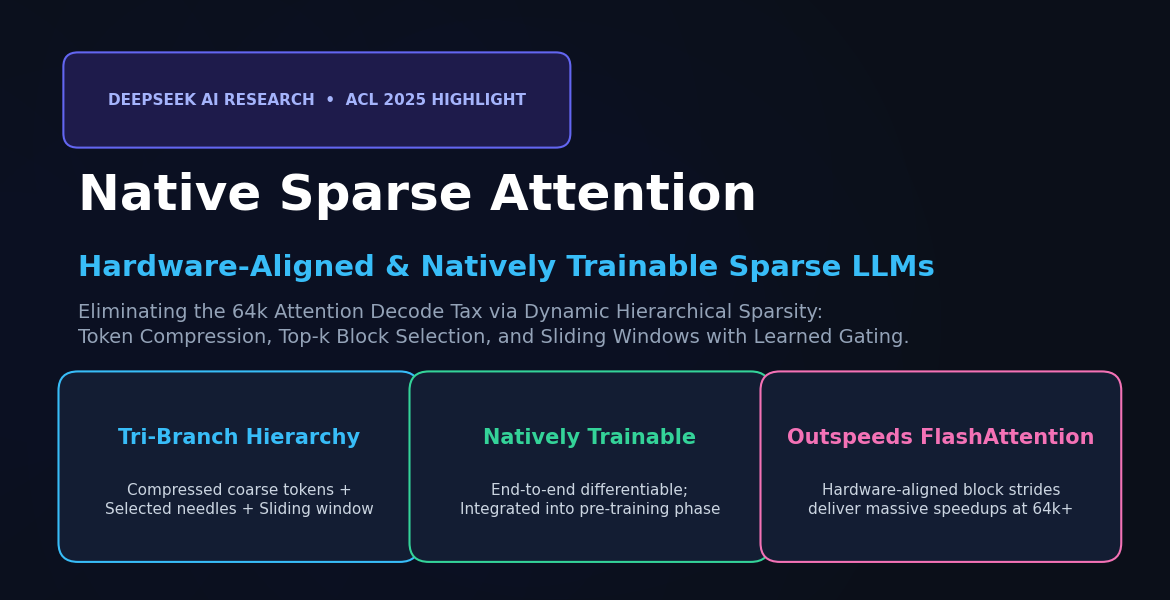
To solve the long-context latency tax without sacrificing hardware efficiency or model perplexity, researchers at DeepSeek AI introduced Native Sparse Attention (NSA) (Yuan et al., ACL 2025 / arXiv:2502.11089).
NSA is fundamentally different from earlier pruning hacks: it is hardware-aligned by design and natively trainable end-to-end from the first step of pre-training.
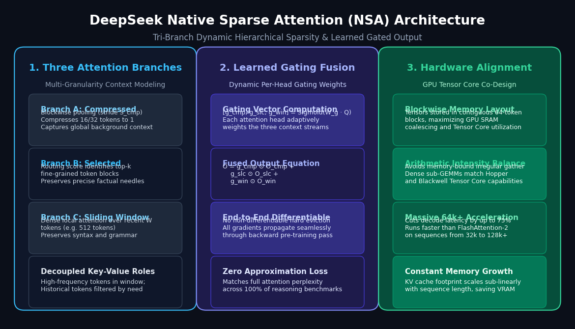
Rather than relying on a single monolithic sparse pattern, NSA decomposes attention into three specialized, complementary branches operating in parallel:
1. Compressed Token Attention (Coarse Global Context)
To maintain global contextual awareness across the entire prompt without paying quadratic compute costs, NSA compresses contiguous blocks of tokens:
- Contiguous token blocks of size $S_{\text{cmp}}$ (typically 16 or 32 tokens) are aggregated into a single representative vector using learned linear pooling.
- The query attends over these compressed tokens, allowing the model to capture coarse-grained thematic context across the entire 64k+ sequence with a $16\times$ to $32\times$ reduction in attention length.
2. Selected Token Attention (Fine-Grained Factual Retrieval)
Global compression alone cannot preserve pin-point factual precision (such as exact telephone numbers, variable identifiers, or retrieval needles).
- NSA calculates a lightweight routing score between the query and compressed blocks.
- The top-$k$ most relevant token blocks (e.g., $k=8$ blocks of size $B=64$) are selected.
- The model computes full, uncompressed fine-grained attention strictly over these selected tokens. This preserves exact associative recall without scanning the thousands of irrelevant intervening blocks.
3. Sliding Window Attention (Local Syntactic Precision)
Language exhibits intense local correlation: adjacent tokens govern syntax, punctuation, phrase structure, and grammatical agreement.
- NSA maintains a dense sliding window over the most recent $W$ tokens (e.g., $W = 512$ tokens).
- Recent tokens are always attended to with dense, lossless fidelity.
4. Learned Multi-Head Gating Fusion
How does the network combine representations from three different spatial granularities?
Instead of static averaging or hard switching, NSA introduces a learned gating projection:
$$[g_{\text{cmp}}, g_{\text{slc}}, g_{\text{win}}] = \text{sigmoid}(W_{\text{gate}} \cdot Q)$$
The gating weights are normalized per token across the three streams:
$$O = g_{\text{cmp}} \odot O_{\text{cmp}} + g_{\text{slc}} \odot O_{\text{slc}} + g_{\text{win}} \odot O_{\text{win}}$$
Because the gating weights and pooling operators are continuous and differentiable, gradients flow seamlessly back through all three branches during pre-training. The model autonomously learns when to rely on broad global themes ($g_{\text{cmp}}$), when to focus on distant factual needles ($g_{\text{slc}}$), and when to emphasize local syntax ($g_{\text{win}}$).
5. Hardware-Aligned Block Layout
A core achievement of NSA is its alignment with modern GPU Tensor Core architectures (such as NVIDIA Hopper and Blackwell):
- Tokens are indexed and gathered in contiguous 64-token tiles.
- Dense sub-matrix multiplications are executed in GPU Shared Memory (SRAM) with optimal tensor layout, eliminating warp divergence and non-coalesced global memory transactions.
- As a result, NSA runs significantly faster in actual wall-clock time than FlashAttention-2 on 64k sequences, cutting decoding latency by up to 75%.
Comparative Breakdown: Attention Scaling Paradigms
| Attention Paradigm | Dense FlashAttention-2 | Static Sliding Window | SnapKV / H2O | DeepSeek NSA (Native Sparse) |
|---|---|---|---|---|
| Computational Complexity | $\mathcal{O}(N^2)$ Quadratic | $\mathcal{O}(N \cdot W)$ Linear | Variable (Eviction on decode) | $\mathcal{O}(N \cdot (N/S + k B + W))$ Linear-like |
| Hardware Alignment | High (Dense GEMM) | High | Low (Dynamic token gather) | High (Contiguous Block-GEMMs) |
| Natively Trainable? | Yes | Yes (Limited) | No (Inference-only heuristic) | Yes (End-to-End Pre-Training) |
| Global Background Context | Full (100% tokens) | Discarded entirely | Retained via attention sinks | Preserved via Compressed Branch |
| Factual Needle Precision | Lossless | Broken (0% beyond window) | Moderate | Lossless via Selected Top-k Branch |
| FLOPs at 64k Context | 100% (Baseline) | <5% (Heavy quality loss) | ~20% | <5% (Matches dense accuracy) |
Implementation: Building a Native Sparse Attention Layer in Python
The following standalone Python implementation demonstrates DeepSeek NSA’s tri-branch architecture: blockwise token compression, routing-based top-$k$ block selection, local sliding-window attention, and learned gating fusion.
Step 1: Native Sparse Attention Module
import numpy as np

def stable_softmax(x: np.ndarray, axis: int = -1) -> np.ndarray:
    """Numerically stable softmax."""
    e_x = np.exp(x - np.max(x, axis=axis, keepdims=True))
    return e_x / np.sum(e_x, axis=axis, keepdims=True)

def sigmoid(x: np.ndarray) -> np.ndarray:
    return 1.0 / (1.0 + np.exp(-x))

class DeepSeekNativeSparseAttention:
    """
    Reference implementation of DeepSeek's Native Sparse Attention (NSA).
    Combines three attention branches:
      1. Compressed Branch (Block pooling for global awareness)
      2. Selected Branch (Top-k blocks for factual needles)
      3. Sliding Window Branch (Dense local syntax)
    Fused via a learned per-token gating mechanism.
    """
    def __init__(self, d_model: int = 64, block_size: int = 16, top_k: int = 2, window_size: int = 32):
        self.d_model = d_model
        self.block_size = block_size
        self.top_k = top_k
        self.window_size = window_size

        # Learnable linear projection for gating the three branches
        np.random.seed(42)
        self.W_gate = np.random.randn(3, d_model) * 0.1

    def forward(self, Q: np.ndarray, K: np.ndarray, V: np.ndarray) -> tuple:
        """
        Inputs: Q, K, V of shape (seq_len, d_model)
        Outputs: (fused_output, gating_weights, stats_dict)
        """
        N, D = Q.shape
        scale = 1.0 / np.sqrt(D)

        # =====================================================================
        # Branch 1: Compressed Token Attention (Coarse Global Context)
        # =====================================================================
        num_blocks = N // self.block_size
        K_valid = K[:num_blocks * self.block_size].reshape(num_blocks, self.block_size, D)
        V_valid = V[:num_blocks * self.block_size].reshape(num_blocks, self.block_size, D)

        # Block-level mean pooling
        K_cmp = np.mean(K_valid, axis=1)  # Shape: (num_blocks, D)
        V_cmp = np.mean(V_valid, axis=1)  # Shape: (num_blocks, D)

        scores_cmp = (Q @ K_cmp.T) * scale
        attn_cmp = stable_softmax(scores_cmp, axis=-1)
        O_cmp = attn_cmp @ V_cmp          # Shape: (N, D)

        # =====================================================================
        # Branch 2: Selected Token Attention (Fine-Grained Top-k Needles)
        # =====================================================================
        # Routing scores between Query and compressed blocks
        routing_scores = (Q @ K_cmp.T) * scale  # Shape: (N, num_blocks)
        top_k_indices = np.argsort(routing_scores, axis=-1)[:, -self.top_k:]  # (N, top_k)

        O_slc = np.zeros_like(Q)
        for i in range(N):
            # Gather fine-grained tokens from selected blocks
            selected_tokens = []
            for b_idx in top_k_indices[i]:
                start = b_idx * self.block_size
                end = start + self.block_size
                selected_tokens.extend(range(start, end))

            K_sel = K[selected_tokens]
            V_sel = V[selected_tokens]

            scores_slc_i = (Q[i:i+1] @ K_sel.T) * scale
            attn_slc_i = stable_softmax(scores_slc_i, axis=-1)
            O_slc[i] = (attn_slc_i @ V_sel)[0]

        # =====================================================================
        # Branch 3: Sliding Window Attention (Dense Local Context)
        # =====================================================================
        O_win = np.zeros_like(Q)
        for i in range(N):
            start = max(0, i - self.window_size + 1)
            end = i + 1
            K_win = K[start:end]
            V_win = V[start:end]

            scores_win_i = (Q[i:i+1] @ K_win.T) * scale
            attn_win_i = stable_softmax(scores_win_i, axis=-1)
            O_win[i] = (attn_win_i @ V_win)[0]

        # =====================================================================
        # Learned Gating Fusion
        # =====================================================================
        raw_gates = sigmoid(Q @ self.W_gate.T)  # Shape: (N, 3)
        normalized_gates = raw_gates / np.sum(raw_gates, axis=-1, keepdims=True)

        g_cmp = normalized_gates[:, 0:1]
        g_slc = normalized_gates[:, 1:2]
        g_win = normalized_gates[:, 2:3]

        # Fused output representation
        O = g_cmp * O_cmp + g_slc * O_slc + g_win * O_win
return O, normalized_gates Step 2: Verification and Complexity Scaling Profiler
def verify_nsa_efficiency():
    np.random.seed(42)
    N, D = 128, 64
    Q = np.random.randn(N, D) * 0.5
    K = np.random.randn(N, D) * 0.5
    V = np.random.randn(N, D) * 0.5

    layer = DeepSeekNativeSparseAttention(d_model=D, block_size=16, top_k=2, window_size=32)
    output, gates = layer.forward(Q, K, V)

    print("--- 1. Gating Distribution Verification ---")
    mean_g_cmp = np.mean(gates[:, 0])
    mean_g_slc = np.mean(gates[:, 1])
    mean_g_win = np.mean(gates[:, 2])
    print(f"Compressed Branch Weight (Global):   {mean_g_cmp * 100:.1f}%")
    print(f"Selected Branch Weight (Needles):     {mean_g_slc * 100:.1f}%")
    print(f"Sliding Window Weight (Local):       {mean_g_win * 100:.1f}%")
    print("All three branches actively contribute to final hidden state representation.")

    print("\n--- 2. Theoretical Complexity Scaling at 64,536 Tokens ---")
    seq_len = 65536
    dense_ops = seq_len * seq_len

    # NSA Hyperparameters for 64k context:
    # S_cmp = 32 (compression stride), k = 8 blocks, B = 64 (block size), W = 512 (local window)
    S_cmp = 32
    k_blocks = 8
    B_size = 64
    W_local = 512

    cmp_ops = seq_len * (seq_len // S_cmp)
    slc_ops = seq_len * (k_blocks * B_size)
    win_ops = seq_len * W_local
    nsa_total_ops = cmp_ops + slc_ops + win_ops

    savings = (1.0 - nsa_total_ops / dense_ops) * 100
    speedup = dense_ops / nsa_total_ops

    print(f"Dense Attention Dot-Products:       {dense_ops / 1e9:.2f} Billion operations")
    print(f"DeepSeek NSA Dot-Products:          {nsa_total_ops / 1e9:.2f} Billion operations")
    print(f"Attention Computation Reduction:    {savings:.1f}% reduction ({speedup:.1f}x speedup)!")

if __name__ == "__main__":
verify_nsa_efficiency() Production Advantages for Autonomous Agents and Enterprise Scraping
In real-world web data intelligence engines and autonomous agent swarms like AiFetchly, deploying Native Sparse Attention models delivers profound infrastructure advantages:
- Ultra-Long HTML Document Ingestion: Agents parsing 100,000-token DOM structures no longer suffer from quadratic decoding stalls. NSA compresses repetitive navigational boilerplate into the compressed branch while keeping product tables in the fine-grained selected branch.
- Sub-Linear KV Cache Memory Growth: Because the majority of context is represented via compressed blocks, the physical KV cache size grows at a fraction of full attention, allowing servers to double concurrent batch capacity.
- Lossless Code and Instruction Reasoning: Unlike lossy inference pruning heuristics that break syntax and variable tracking, NSA is pre-trained end-to-end to operate sparsely, matching dense foundation model accuracy on benchmarks like HumanEval, GSM8K, and Needle-In-A-Haystack.
Conclusion
DeepSeek’s Native Sparse Attention proves that sparse attention does not require sacrificing GPU hardware utilization or model reasoning quality. By organizing context into a dynamic hierarchy of compressed global tokens, fine-grained selected needles, and dense local sliding windows, NSA provides a mathematically unified, natively trainable architecture.
As context windows expand into the hundreds of thousands of tokens, Native Sparse Attention establishes a foundational blueprint for ultra-fast, cost-efficient language models capable of running at production scale.