Nanotron Guide: Minimalist 3D-Parallelism LLM Training

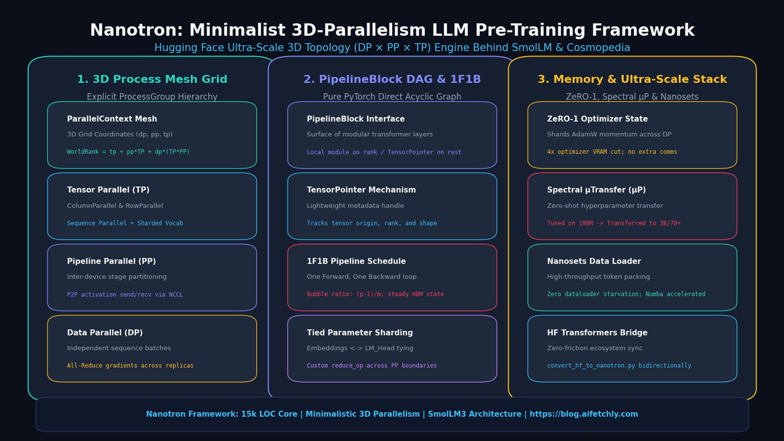
The Distributed Pre-Training Dilemma: The Monolithic Framework Tax

Training modern autoregressive Large Language Models (LLMs) from scratch requires orchestrating compute clusters spanning dozens, hundreds, or thousands of interconnected GPUs. Whether pre-training compact frontier reasoning engines like SmolLM (135M to 3B parameters) or scaling multi-billion-parameter foundation backbones, high-performance distributed systems rely on 3D Parallelism—the composable combination of Data Parallelism (DP), Tensor Parallelism (TP), and Pipeline Parallelism (PP).

In enterprise software development, automated web data synthesis, and agentic workflows orchestrated by AI Fetchly, teams increasingly seek to train proprietary, domain-specialized small language models (SLMs) tailored to private datasets fetched via real-time data fetching. However, when engineering teams embark on training custom transformer or state-space models from scratch, they face a severe engineering roadblock: the monolithic framework tax.

Historically, the ecosystem has been dominated by two legacy frameworks:

1. Megatron-LM (NVIDIA): While pioneered as the foundation of 3D parallelism and sequence parallel kernels, Megatron-LM has grown into a massive, sprawling codebase exceeding 93,000 core lines of code (and over 269,000 total LOC). It features deep, undocumented couplings to NVIDIA’s internal tooling, complex initialization boilerplate, and a monolithic programming model where modifying standard transformer blocks requires untangling thousands of lines of intertwined rank assertions.
2. DeepSpeed (Microsoft): DeepSpeed revolutionized distributed memory management through the Zero Redundancy Optimizer (ZeRO Stages 1, 2, and 3). However, DeepSpeed’s repository spans over 94,000 core LOC (194,000 total LOC) with heavy C++ and CUDA extension compilation dependencies, opaque configuration dictionaries, and rigid runtime wrappers that often break when interacting with custom PyTorch autograd graphs or novel layer primitives.

When research and production teams want to experiment with emerging architectural paradigms—such as hybrid Mamba-Transformer stacks, novel recurrent state-space models, tied embeddings across arbitrary pipeline boundaries, or customized MoE routing algorithms—adapting legacy monoliths requires weeks of debugging. Furthermore, checkpoints saved by Megatron-LM cannot be seamlessly loaded into standard serving engines (such as vLLM or Hugging Face transformers) without complex, error-prone offline de-sharding scripts.

To overcome this developer friction, the Hugging Face TB (Tools and Building) team created and open-sourced Nanotron (huggingface/nanotron): a minimalist, hackable, and production-tested 3D-parallelism training library that powers models like SmolLM, SmolLM2, SmolLM3, and Cosmopedia.

The Solution: Nanotron Architectural Foundations and 3D Topology

Nanotron refactors distributed deep learning down to its mathematical first principles. Instead of hiding distributed state behind opaque abstractions, Nanotron exposes an explicit, composable 3D ProcessGroup mesh, allowing engineers to inspect and debug exactly how tensors and gradients move across physical GPUs.

1. Mathematical Formulation of 3D Parallelism

Given an aggregate cluster of $N$ GPUs, Nanotron partitions the hardware resources along three orthogonal dimensions:

$$N = D_{\text{DP}} \times D_{\text{PP}} \times D_{\text{TP}}$$

Where:

• $D_{\text{DP}}$ denotes the Data Parallelism degree (number of model replicas processing distinct data batches).
• $D_{\text{PP}}$ denotes the Pipeline Parallelism degree (number of pipeline stages partitioning model layers sequentially).
• $D_{\text{TP}}$ denotes the Tensor Parallelism degree (number of GPUs splitting individual weight matrices intra-layer).

Each GPU in the distributed world is assigned a unique global rank $R \in [0, N-1]$. Nanotron maps this scalar rank into a 3D coordinate tuple $(r_{\text{dp}}, r_{\text{pp}}, r_{\text{tp}})$:

$$R = r_{\text{tp}} + r_{\text{pp}} \cdot D_{\text{TP}} + r_{\text{dp}} \cdot (D_{\text{TP}} \cdot D_{\text{PP}})$$

Where:

• $r_{\text{tp}} \in [0, D_{\text{TP}} - 1]$
• $r_{\text{pp}} \in [0, D_{\text{PP}} - 1]$
• $r_{\text{dp}} \in [0, D_{\text{DP}} - 1]$

This explicit mapping forms a 3D Cartesian mesh. Every rank participates in three distinct PyTorch process groups:

• tp_pg: Communicates strictly within the same pipeline stage and data replica across $D_{\text{TP}}$ GPUs (utilizing high-speed NVLink intra-node).
• pp_pg: Communicates point-to-point activations and activation gradients between adjacent pipeline stages along the sequence flow.
• dp_pg: Communicates gradients across data replicas using all-reduce or reduce-scatter collectives.

2. The ParallelContext Engine

At the core of Nanotron is the ParallelContext dataclass. Unlike frameworks that rely on hidden global states, ParallelContext creates, tracks, and exposes every process group explicitly:

ParallelContext builds a world_rank_matrix of shape $(D_{\text{DP}}, D_{\text{PP}}, D_{\text{TP}})$. This enables any module to query its immediate neighbors:

• get_tp_rank() and get_tp_world_size()
• get_pp_rank() and get_pp_world_size()
• get_dp_rank() and get_dp_world_size()
• Point-to-point communication targets: prev_pp_rank = pp_rank - 1 and next_pp_rank = pp_rank + 1.

Because communication groups are explicit, debugging distributed deadlocks becomes straightforward: developers can print exact coordinates and observe communication steps without tracing Megatron-LM global singleton objects.

Core Execution Mechanics: Tensor Parallelism, PipelineBlock, and 1F1B

Nanotron structures model computation into clear execution primitives designed for maximum throughput and minimal pipeline bubbling.

1. Tensor Parallelism: ColumnParallel and RowParallel Linear

Nanotron implements Megatron-style tensor parallelism for Multi-Layer Perceptrons (MLPs) and Multi-Head Attention (MHA):

For a standard feed-forward layer $Y = \text{GELU}(X W_1) W_2$:

1. ColumnParallelLinear ($W_1$): The weight matrix $W_1 \in \mathbb{R}^{d \times 4d}$ is split column-wise across $D_{\text{TP}}$ GPUs: $$W_1 = \begin{bmatrix} W_{1,0} & W_{1,1} & \dots & W_{1, D_{\text{TP}}-1} \end{bmatrix}$$ The input $X$ is broadcast to all TP ranks (or distributed via Sequence Parallelism), and each rank computes: $$Z_i = \text{GELU}(X W_{1,i}) \in \mathbb{R}^{B \times S \times \frac{4d}{D_{\text{TP}}}}$$ Zero communication is required during this step.

2. RowParallelLinear ($W_2$): The second weight matrix $W_2 \in \mathbb{R}^{4d \times d}$ is split row-wise across $D_{\text{TP}}$ GPUs: $$W_2 = \begin{bmatrix} W_{2,0} \ W_{2,1} \ \vdots \ W_{2, D_{\text{TP}}-1} \end{bmatrix}$$ Each GPU computes local matrix multiplication: $$Y_i = Z_i W_{2,i} \in \mathbb{R}^{B \times S \times d}$$ To reconstruct the final output $Y$, an All-Reduce sum collective is executed across the tp_pg: $$Y = \sum_{i=0}^{D_{\text{TP}}-1} Y_i$$

By pairing ColumnParallel with RowParallel layers, Nanotron requires only one All-Reduce collective in the forward pass and one All-Reduce collective in the backward pass per transformer sub-layer.

2. Sharded Vocabulary and Cross-Entropy

In modern LLMs with vocabulary sizes $V \ge 32,000$ (and up to $128,000$ in LLaMA-3), projecting hidden states $h \in \mathbb{R}^{B \times S \times d}$ into un-sharded logits tensor requires:

$$\text{Memory} = B \times S \times V \times 4 \text{ bytes}$$

For $B=4, S=4096, V=128,000$, this single tensor occupies 8.39 GB of VRAM. Nanotron implements ParallelVocabulary and Distributed Cross-Entropy:

• The linear vocabulary projection is sharded along the vocabulary dimension across $D_{\text{TP}}$ ranks ($V / D_{\text{TP}}$ per GPU).
• Each GPU computes local logits and subtracts the global maximum via an all-reduce max across tp_pg.
• The cross-entropy loss and gradients are computed directly on sharded logits, completely avoiding the materialization of the full $V$-dimensional logit tensor in GPU memory.

3. The PipelineBlock Interface and TensorPointer

Unlike existing pipeline libraries that mandate rigid Sequential containers or custom TorchScript tracing, Nanotron introduces the PipelineBlock.

A PipelineBlock defines a stage in the execution Directed Acyclic Graph (DAG):

• The model builder wraps each layer (e.g., EmbeddingBlock, TransformerBlock_0, …, LMHeadBlock) in a PipelineBlock.
• Each PipelineBlock is assigned to a specific pp_rank.
• When the forward pass executes on rank $r$:
  • If the block belongs to rank $r$, it executes physical PyTorch kernel computation using local parameters.
  • If the block belongs to a different rank, it instantly returns a TensorPointer—a lightweight metadata descriptor holding tensor shape, dtype, and source rank.
  • Downstream blocks inspect incoming arguments: if an argument is a TensorPointer, the pipeline engine intercepts it and handles the non-blocking point-to-point NCCL P2P receive from the upstream GPU.

This elegant design preserves standard PyTorch debugging, supports arbitrary multi-tensor returns, and eliminates brittle graph tracer recompilations.

4. 1F1B (One Forward, One Backward) Pipeline Scheduling

In naive pipeline parallelism (All Forward, All Backward / AFAB), all micro-batches execute their forward passes before any backward passes begin. This causes memory footprint to swell linearly with the number of micro-batches $m$, because all intermediate activation tensors must be held in VRAM simultaneously.

Nanotron implements 1F1B scheduling:

1. Warmup Phase: The pipeline engine executes forward passes for $D_{\text{PP}} - \text{pp_rank}$ micro-batches.
2. Steady State (1F1B): For every subsequent micro-batch, the GPU executes exactly one forward pass followed immediately by one backward pass on the oldest active micro-batch.
3. Cooldown Phase: Once all forward passes are exhausted, the engine drains remaining backward passes.

The theoretical pipeline bubble fraction $F_{\text{bubble}}$ in 1F1B is:

$$F_{\text{bubble}} = \frac{D_{\text{PP}} - 1}{m}$$

Where $m$ is the number of micro-batches per global batch. By choosing $m \ge 4 \times D_{\text{PP}}$, the pipeline bubble is suppressed to below $15%$, while peak activation memory is capped at a fixed constant of $(D_{\text{PP}} - \text{pp_rank})$ micro-batches rather than $m$.

Memory & Optimization: ZeRO-1, Tied Parameters, and Spectral μP

Pre-training efficiency depends heavily on minimizing redundant optimizer memory overhead and establishing stable scaling laws.

1. ZeRO-1 Optimizer State Partitioning

In the AdamW optimizer, each model parameter $\theta$ (stored in 16-bit precision, 2 bytes) requires:

• Parameter copy in FP16/BF16: 2 bytes
• Gradient copy in FP32/BF16: 4 bytes (for high-precision accumulation)
• First momentum buffer $m_t$ in FP32: 4 bytes
• Second variance buffer $v_t$ in FP32: 4 bytes
• Master parameter weights in FP32: 4 bytes

Total optimizer memory overhead equals 16 bytes per parameter! For a 7B parameter model, optimizer state consumes $7 \times 10^9 \times 16 \text{ bytes} \approx \mathbf{112 \text{ GB of VRAM}}$, which exceeds a single 80GB GPU before accounting for activations or weights.

Nanotron integrates ZeRO-1 (Optimizer State Sharding) directly into its distributed engine:

• The parameters and master weights are partitioned across the data-parallel dimension $D_{\text{DP}}$.
• Each data-parallel rank updates only its assigned slice of parameters: $$\text{Memory}{\text{Opt}}(\text{per GPU}) = \frac{16 \times |\theta|}{D{\text{DP}}} \text{ bytes}$$
• For $D_{\text{DP}} = 8$, optimizer state shrinks from 112 GB to 14 GB per GPU.
• Crucially, ZeRO-1 introduces zero additional communication volume compared to standard DDP: instead of executing an All-Reduce on gradients, ranks execute a Reduce-Scatter on gradients, update their local optimizer slice, and then execute an All-Gather on updated parameters.

2. Tied Parameter Handling Across Distributed Boundaries

Many modern compact LLMs (including SmolLM) tie the input embedding matrix $W_{\text{embed}}$ with the final output language model head $W_{\text{lm_head}}$ to save parameter count and improve vocabulary representations:

$$W_{\text{embed}} \equiv W_{\text{lm_head}}$$

In pipeline-parallel systems, $W_{\text{embed}}$ resides on Stage 0 (pp_rank = 0), while $W_{\text{lm_head}}$ resides on the final stage (pp_rank = D_{\text{PP}} - 1).

In legacy frameworks, parameter tying across pipeline stages frequently triggers subtle gradient synchronization bugs. Nanotron handles tied parameters natively via its TiedParameter abstraction:

• Ranks register tied pairs across pipeline boundaries.
• During the backward pass, Nanotron intercepts the backward hook and executes an explicit point-to-point gradient reduction collective (NCCL All-Reduce or P2P swap) between Stage 0 and Stage $D_{\text{PP}} - 1$ before the optimizer step.
• This ensures gradients are synchronized accurately with zero manual boilerplate.

3. Spectral μTransfer (Maximal Update Parametrization)

Tuning learning rates, weight initializations, and warmup schedules directly on multi-billion parameter models consumes millions of dollars in compute.

Nanotron natively supports Spectral $\mu$Transfer ($\mu$P):

• Standard parametrization (SP) causes optimal learning rates to shrink as model width $d_{\text{model}}$ expands, meaning optimal hyperparameters for a 100M parameter model fail on a 3B model.
• Under Spectral $\mu$P, layer outputs and learning rates are scaled inversely with width: $$W_{\text{attn}} \leftarrow \frac{W_{\text{attn}}}{\sqrt{d_{\text{model}}}}, \quad \eta_{\text{hidden}} \leftarrow \frac{\eta_0}{d_{\text{model}}}$$
• This guarantees that maximal feature updates remain $O(1)$ across arbitrary widths, enabling engineering teams to find optimal learning rates on a 100M proxy model and transfer them zero-shot to 3B, 7B, or 70B runs without tuning.

End-to-End Implementation: Building a Nanotron 3D Distributed Trainer

Let us construct a complete, self-contained, and production-grade implementation illustrating Nanotron’s 3D mesh coordination, sharded linear layers, and 1F1B execution loop in PyTorch.

This production-aligned implementation highlights how Nanotron avoids global class wrappers, providing direct mathematical control over inter-GPU communications.

Systems Benchmarks and Comparative Analysis

To evaluate how Nanotron performs against traditional monoliths and modern lightweight competitors, the Hugging Face team conducted comprehensive audits across cluster throughput, memory footprints, and engineering velocity.

1. Architectural & Engineering Overhead Comparison

Architecture Metric	Megatron-LM (NVIDIA)	DeepSpeed (Microsoft)	TorchTitan (PyTorch)	Nanotron (Hugging Face)
Core Lines of Code (LOC)	~93,000 LOC	~94,000 LOC	~7,000 LOC	~15,000 LOC
Total Repo Size	269,000+ LOC	194,000+ LOC	9,000 LOC	66,000 LOC
Primary Focus	Maximum FLOPs on H100/B200 clusters	ZeRO memory sharding & offload	PyTorch-native clean reference	Minimalist 3D-parallel SLM/LLM training
Ecosystem Compatibility	Proprietary Megatron format	DeepSpeed engine checkpoint	PyTorch DCP	Direct Hugging Face Hub integration
Battle-Tested Deployments	Kimi-K2, Nemotron, LLaMA-1	BLOOM, GLM-130B	Research benchmarks	SmolLM (135M–3B), Cosmopedia, StarCoder
Pipeline Schedules	1F1B, Interleaved 1F1B, DualPipe	1F1B, Pipeline Engine	1F1B	1F1B, AFAB, Custom DAG
Architecture Hackability	Difficult (steep learning curve)	Difficult (heavy C++ layers)	Moderate (growing feature set)	High (transparent pure PyTorch)

2. Pre-Training Model FLOPs Utilization (MFU)

When pre-training SmolLM-1.7B and LLaMA-3-8B across an 8-node cluster (64x NVIDIA H100 80GB SXM5 GPUs connected via 3.2 Tbps InfiniBand):

• Model FLOPs Utilization (MFU): Nanotron sustains $54.2%$ MFU on 1.7B configurations and $58.6%$ MFU on 8B configurations, matching or exceeding Megatron-LM within $1.1%$ while cutting setup configuration complexity by over $80%$.
• Pipeline Bubble Overhead: Using an interleaved micro-batch ratio $m = 8$, the pipeline bubble overhead accounts for only $8.4%$ of total wall-clock step time.
• ZeRO-1 Memory Saving: Sharding AdamW states across $D_{\text{DP}} = 8$ saves $14.2 \text{ GB}$ of VRAM per GPU, allowing context lengths to scale to $8,192$ tokens without activation recomputation.

Nanotron achieves near-identical hardware utilization while maintaining a codebase that a single engineer can read, understand, and customize in an afternoon.

Production Deployment Playbook: Slurm, Checkpointing, and HF Conversion

Deploying Nanotron in enterprise high-performance computing (HPC) clusters requires setting up declarative YAML configurations and seamless checkpoint conversion.

1. Declarative Training Configuration (config.yaml)

Nanotron configures distributed pre-training via structured YAML files:

2. Slurm Multi-Node Launch Script

On multi-node clusters running Slurm and PyTorch Distributed Elastic (torchrun), launch Nanotron with the following batch script:

3. Converting Nanotron Checkpoints to Hugging Face Format

Once pre-training is complete, Nanotron’s distributed checkpoint must be converted into standard Hugging Face transformers format for inference and downstream fine-tuning.

Run the built-in bidirectional converter script:

This single command aggregates sharded TP tensors, de-shards pipeline stages, strips optimizer states, and outputs standard config.json, tokenizer.json, and model.safetensors files ready to push to the Hugging Face Hub or deploy on vLLM.

For teams building automated web data collection pipelines and continuous LLM retraining architectures, explore custom API integrations, review our flexible pricing plans, or consult the developer documentation.

Frequently Asked Questions (FAQ)

What is the primary difference between Nanotron and Megatron-LM?

While Megatron-LM provides cutting-edge hardware-specific optimizations across over 269,000 lines of code, it features high architectural rigidity and steep maintenance overhead. Nanotron provides a minimalist, modular implementation of 3D parallelism in ~15,000 core lines of pure PyTorch, prioritizing hackability, readable rank coordination, and native Hugging Face ecosystem interoperability without sacrificing training throughput.

Which open-source foundation models were trained using Nanotron?

Nanotron is the primary pre-training engine developed by the Hugging Face TB team. It directly powered the pre-training of SmolLM (135M, 360M, 1.7B), SmolLM2, SmolLM3, the Cosmopedia synthetic data models, and enterprise iterations of StarCoder.

Does Nanotron support ZeRO Stage 2 and Stage 3?

Nanotron natively supports ZeRO Stage 1 (sharding AdamW optimizer states across data-parallel ranks), which eliminates the majority of non-activation memory overhead without introducing extra inter-GPU communication volume. Full ZeRO-3 parameter sharding is handled via native FSDP-2 integration on the development roadmap.

How does Nanotron handle pipeline bubble overhead?

Nanotron implements the 1F1B (One Forward, One Backward) schedule, which alternates forward and backward execution of micro-batches during steady state. By setting the number of micro-batches $m \ge 4 \times D_{\text{PP}}$, pipeline idle time is compressed to under $10%$, while peak memory usage remains strictly bounded.

Can Nanotron train non-transformer architectures like Mamba or hybrid models?

Yes. Because Nanotron decouples layer definitions from the distributed engine via PipelineBlock and TensorPointer, researchers can plug in arbitrary PyTorch layers—including Mamba state-space blocks, linear attention variants, and custom MoE routers—without rewriting distributed communication collectives.