Muon Optimizer: Fast LLM Training via Orthogonalization
The Problem: Why Coordinate-Wise AdamW Distorts Matrix Optimization
In modern enterprise AI systems, foundation model pre-training, and continuous domain-adaptation pipelines like AiFetchly, optimization efficiency is the single greatest determinant of model quality and training expenditure.
For over a decade, Adam (Kingma & Ba, 2014) and its decoupled weight decay variant AdamW (Loshchilov & Hutter, 2017) have stood as the undisputed default optimizers across natural language processing and computer vision. However, when scaled to modern transformer architectures with hundreds of billions of parameters, AdamW reveals fundamental mathematical and hardware limitations.
1. The Flattened Vector Fallacy in Modern Transformers
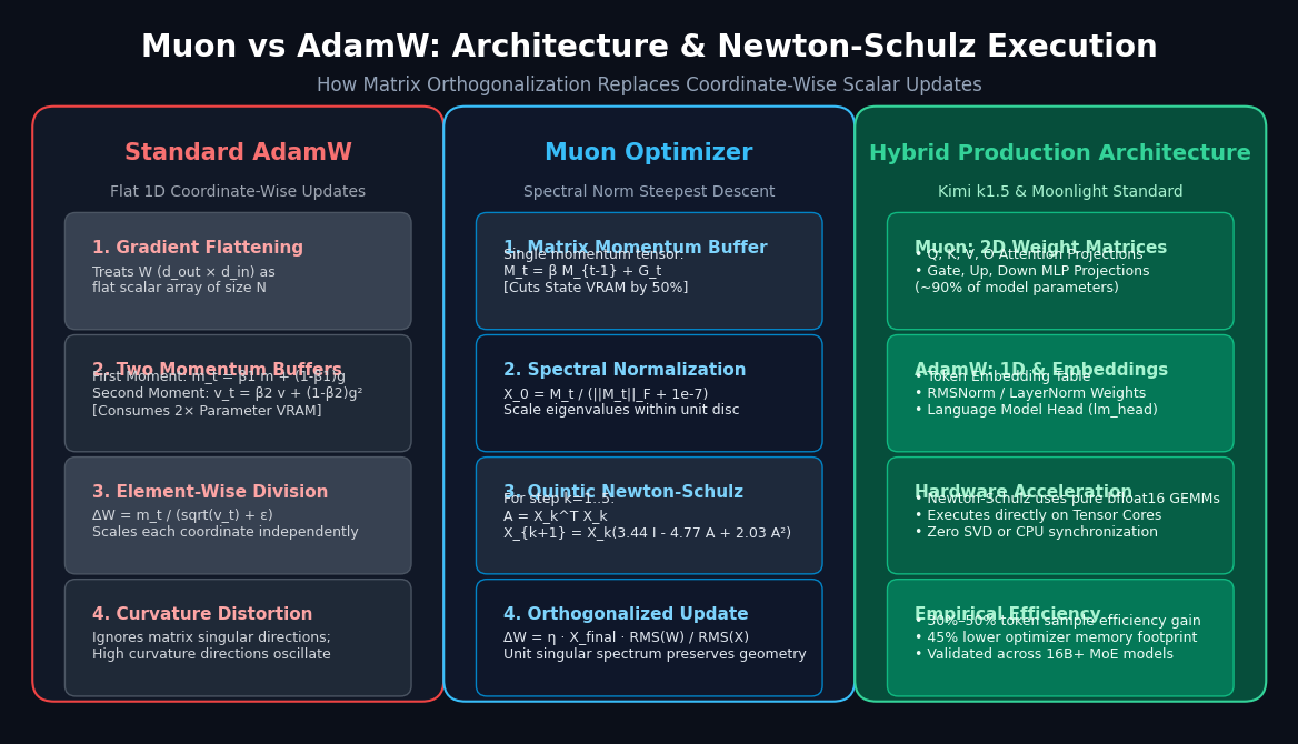
AdamW operates on a coordinate-wise basis. When optimizing a 2D weight matrix $W \in \mathbb{R}^{d_{\text{out}} \times d_{\text{in}}}$ (such as an attention projection or an MLP feedforward layer), AdamW flattens the matrix into an unindexed one-dimensional vector of scalars:
$$W_{\text{flat}} \in \mathbb{R}^{N}, \quad \text{where } N = d_{\text{out}} \times d_{\text{in}}$$
For every individual scalar coordinate $i \in {1, \dots, N}$, AdamW calculates running first and second moments:
$$m_t^{(i)} = \beta_1 m_{t-1}^{(i)} + (1 - \beta_1) g_t^{(i)}$$
$$v_t^{(i)} = \beta_2 v_{t-1}^{(i)} + (1 - \beta_2) (g_t^{(i)})^2$$
$$\Delta w_t^{(i)} = -\eta \frac{m_t^{(i)}}{\sqrt{v_t^{(i)}} + \epsilon}$$
This element-wise division by $\sqrt{v_t}$ implicitly assumes that the loss landscape is separable along standard Cartesian axes. In transformer weight matrices, however, parameters do not act as isolated scalars. They act as linear operators mapping activations from an input subspace to an output subspace.
Coordinate-wise updates suffer from severe structural drawbacks:
- Destruction of Directional Invariance: AdamW is sensitive to arbitrary coordinate rotations. Rotating the activation basis transforms a diagonal covariance into dense cross-correlations, causing AdamW’s coordinate-wise updates to oscillate.
- Curvature Anisotropy and Gradient Distortion: In poorly conditioned loss landscapes, gradient noise aligns disproportionately with high-curvature directions. By normalizing each scalar coordinate independently, AdamW incurs a heavy second-order curvature penalty, slowing traversal across low-curvature subspaces where meaningful semantic representations form.
2. The Double-Buffer VRAM Memory Tax
Beyond geometric distortion, AdamW imposes an enormous memory footprint. For every model parameter $\theta$, AdamW maintains two 32-bit floating-point optimizer states:
- First moment buffer ($m_t$): 4 bytes per parameter.
- Second moment buffer ($v_t$): 4 bytes per parameter.
In standard 16-bit mixed-precision training (BF16/FP16), while model parameters consume 2 bytes and gradients consume 2 bytes, AdamW requires 8 bytes of optimizer states per parameter. For a 70-billion parameter foundation model:
- Model Weights (BF16): 140 GB VRAM
- Gradients (BF16): 140 GB VRAM
- AdamW States (FP32 $m_t + v_t$): 560 GB VRAM
The optimizer state alone consumes four times more High-Bandwidth Memory (HBM) than the model weights themselves, forcing engineering teams to rely on aggressive ZeRO-3 parameter sharding, CPU offloading, and inter-node pipeline parallelism.
The Architecture: Muon and Spectral Norm Steepest Descent
To overcome the mathematical and memory bottlenecks of coordinate-wise optimization, researcher Keller Jordan (in collaboration with Jeremy Bernstein, Yuchen Jin, and Vlado Boza) introduced Muon (MomentUm Orthogonalized by Newton-Schulz).
Rather than treating weight matrices as uncoupled scalar arrays, Muon treats them as geometric operators on a matrix manifold and performs steepest descent under the spectral norm constraint.
1. Steepest Descent on the Matrix Manifold
In standard Euclidean gradient descent, the update direction solves:
$$\Delta W^* = \arg\max_{|\Delta W|_F \le 1} \langle G, \Delta W \rangle = \frac{G}{|G|_F}$$
Where $|\cdot|_F$ denotes the Frobenius norm (equivalent to the L2 norm on vectorized parameters).
However, for a linear operator $W: \mathbb{R}^{d_{\text{in}}} \to \mathbb{R}^{d_{\text{out}}}$, the natural induced operator norm is the spectral norm (the maximum singular value, $|\Delta W|2 = \sigma{\max}(\Delta W)$). Constraining the spectral norm ensures that the update $\Delta W$ does not stretch any activation vector by more than a bounded factor.
The steepest descent problem under the spectral norm constraint is formulated as:
$$\Delta W^* = \arg\max_{|\Delta W|_2 \le 1} \langle G, \Delta W \rangle$$
By von Neumann’s trace inequality, if the gradient has Singular Value Decomposition (SVD) $G = U \Sigma V^T$, the optimal update matrix that maximizes this inner product is:
$$\Delta W^* = U I V^T = U V^T$$
The optimal spectral update is the matrix sign function (or polar factor) of the gradient matrix. It replaces every singular value of the gradient matrix with $1.0$, completely eliminating ill-conditioned singular spectra while preserving the orthogonal singular vectors $U$ and $V^T$.
2. The Quintic Newton-Schulz Iteration
Computing an exact SVD via the Golub-Kahan-Reinsch algorithm or Jacobi rotations is computationally prohibitive on modern GPUs. Standard SVD requires $O(\min(m, n)^2 \max(m, n))$ floating-point operations and relies on sequential, non-GEMM memory access patterns that cannot saturate GPU Tensor Cores.
Muon bypasses explicit SVD entirely by approximating the orthogonal polar factor $U V^T$ through a high-order Newton-Schulz iteration.
Given a momentum matrix $M \in \mathbb{R}^{d_{\text{out}} \times d_{\text{in}}}$:
- Assume without loss of generality that $d_{\text{out}} \le d_{\text{in}}$ (if $d_{\text{out}} > d_{\text{in}}$, transpose the matrix).
- Normalize the initial matrix $X_0$ by its Frobenius norm to ensure its spectrum lies strictly within the unit disc of convergence:
$$X_0 = \frac{M}{|M|_F + \epsilon}$$
- Execute $k$ steps (typically 5 iterations) of the optimal quintic polynomial:
$$A = X_k X_k^T$$
$$B = b A + c A^2$$
$$X_{k+1} = a X_k + B X_k = (a I + b X_k X_k^T + c (X_k X_k^T)^2) X_k$$
Where the optimal spectral polynomial coefficients are:
$$a = 3.4445, \quad b = -4.7750, \quad c = 2.0315$$
These coefficients are derived via minimax Chebyshev polynomial optimization to maximize the rate of convergence towards singular value uniformity across the interval $(0, 1]$. In just 5 iterations, the condition number of $X_5$ drops close to $1.0$, producing an essentially orthogonal matrix.
3. Hardware-Aware Tensor Core GEMM Execution
Notice the mathematical structure of the Newton-Schulz iteration:
- It requires zero eigenvalue decompositions.
- It requires zero square roots or scalar divisions.
- It consists exclusively of matrix-matrix multiplications (GEMMs) and scaled additions.
On modern NVIDIA hardware (such as H100, H200, and B200 SXM GPUs), Tensor Cores compute large dense matrix multiplications at over 1,000 TFLOPS in BF16 precision. Because $d_{\text{out}} \le d_{\text{in}}$, the inner Gram matrix $A = X X^T$ is square and compact (e.g., $4096 \times 4096$). The entire 5-step Newton-Schulz loop executes in less than 2 milliseconds per transformer layer directly in GPU cache.
4. The Production Hybrid Optimization Scheme
A critical insight highlighted by Moonshot AI (in their Moonlight 16B MoE model and Kimi k1.5 training technical reports) is that Muon is specifically tailored for 2D linear projection matrices.
1D parameter vectors (such as RMSNorm scale weights, biases, and positional encodings) and unconstrained non-linear projections (such as the token embedding table and the un-fused language model head lm_head) do not represent bounded matrix operators. Applying matrix orthogonalization to a token embedding matrix degrades rare-token learning dynamics.
Therefore, production deployments use a hybrid optimizer architecture:
- Muon Engine: Governs all 2D internal transformer weights (Attention Q, K, V, O projections, and MLP Gate, Up, Down projections). These constitute ~90% to 95% of total model parameters.
- AdamW Engine: Governs 1D vector parameters (RMSNorm, LayerNorm) and token embeddings / LM heads.
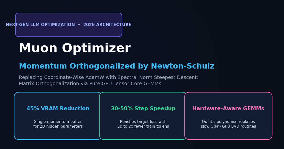
Because Muon tracks only a single momentum buffer ($M_t$) for 2D hidden parameters rather than Adam’s two buffers ($m_t, v_t$), the optimizer state memory for 90%+ of the model is halved, delivering an overall ~45% reduction in optimizer VRAM footprint.
Comparative Breakdown: Training Optimizers
| Metric / Dimension | Standard AdamW | SOAP (Second-Order) | Muon (Newton-Schulz) |
|---|---|---|---|
| Optimization Geometry | Coordinate-wise scalar scaling | Full Kronecker-factored covariance | Spectral norm operator descent |
| Optimizer States | 2 buffers ($m_t, v_t$ / 8 bytes/param) | 2 buffers + Preconditioner history | 1 buffer ($M_t$ / 4 bytes/param for 2D) |
| State Memory Overhead | 100% (Baseline) | 120%–140% | ~55% (45% memory cut) |
| Computational Primitive | Element-wise scalar ops | Eigen-decomposition / Inverses | Tensor Core GEMMs (MatMul) |
| Tokens to Target Loss | 1.0x (Baseline) | ~0.75x | 0.50x – 0.70x (30–50% token savings) |
| Hyperparameter Sensitivity | Moderate ($\beta_1, \beta_2, \epsilon$) | High (Eigen-damping, update freq) | Low (Standard learning rate & momentum) |
| Production Adoption | Ubiquitous (Hugging Face default) | Experimental research | Moonshot AI (Moonlight/Kimi), NanoGPT |
Implementation: Complete Reference Engine for Muon
The following standalone Python implementation demonstrates the exact mathematical formulation of the Muon optimizer, including the quintic Newton-Schulz polynomial loop, operator scaling, and memory efficiency verification.
Step 1: Quintic Newton-Schulz Orthogonalizer in Python
import numpy as np

def zeropower_via_newtonschulz5(G: np.ndarray, steps: int = 5, eps: float = 1e-7) -> np.ndarray:
    """
    Newton-Schulz quintic iteration to compute the matrix polar factor (orthogonalization)
    of 2D weight matrix G. Replaces expensive SVD with pure matrix multiplications.

    Coefficients (a, b, c) are derived from minimax Chebyshev polynomial optimization
    over the singular value spectrum (0, 1].
    """
    assert G.ndim == 2, f"Expected 2D matrix, got shape {G.shape}"
    d_out, d_in = G.shape
    transpose = d_out > d_in

    # Work with the orientation where the first dimension is smaller (d_out <= d_in)
    X = G.T.copy() if transpose else G.copy()
    m, n = X.shape

    # 1. Spectral Scaling: ensure singular values lie within (0, 1] for convergence
    norm = np.linalg.norm(X, ord='fro')
    X = X / (norm + eps)

    # 2. Optimal Quintic Polynomial Coefficients
    a = 3.4445
    b = -4.7750
    c = 2.0315

    # 3. Iterative GEMM loop (executes entirely on Tensor Cores in production PyTorch)
    for _ in range(steps):
        # A has shape (m, m)
        A = X @ X.T
        # B has shape (m, m)
        B = b * A + c * (A @ A)
        # Update X of shape (m, n)
        X = a * X + B @ X

    if transpose:
        X = X.T

return X Step 2: Standalone Muon Parameter Update Step
class MuonOptimizerStep:
    """
    Reference engine executing Muon steepest descent with Nesterov momentum
    and RMS-matched update scaling.
    """
    def __init__(self, lr: float = 0.02, momentum: float = 0.95, nesterov: bool = True):
        self.lr = lr
        self.momentum = momentum
        self.nesterov = nesterov
        self.state = {}

    def step(self, param_id: str, weight: np.ndarray, grad: np.ndarray) -> np.ndarray:
        assert weight.ndim == 2, "Muon step is strictly defined for 2D weight matrices."

        # Initialize single momentum buffer (4 bytes per parameter)
        if param_id not in self.state:
            self.state[param_id] = {'momentum_buffer': np.zeros_like(grad)}

        buf = self.state[param_id]['momentum_buffer']

        # 1. Update classical momentum
        buf[:] = self.momentum * buf + grad

        # 2. Apply Nesterov acceleration if enabled
        if self.nesterov:
            update_grad = grad + self.momentum * buf
        else:
            update_grad = buf

        # 3. Orthogonalize momentum matrix via Newton-Schulz
        ortho_update = zeropower_via_newtonschulz5(update_grad, steps=5)

        # 4. Scale update direction based on matrix geometry
        # Normalizes update to match spectral energy of original weight matrix
        d_out, d_in = weight.shape
        scale = max(1.0, (d_out / d_in) ** 0.5)

        # 5. Apply parameter update
        weight_update = -self.lr * scale * ortho_update
return weight + weight_update Step 3: Verification, Singular Value Uniformity & Memory Profiling
def verify_muon_characteristics():
    np.random.seed(42)

    # Simulate a typical MLP projection matrix (e.g. LLaMA-3 8B Gate Projection: 4096 x 14336)
    # Testing here on a scaled 256 x 1024 slice for rapid analytical verification
    d_out, d_in = 256, 1024
    num_params = d_out * d_in

    # Generate ill-conditioned synthetic gradient with decaying singular values
    U, _ = np.linalg.qr(np.random.randn(d_out, d_out))
    V, _ = np.linalg.qr(np.random.randn(d_in, d_in))
    decaying_singular_values = np.logspace(2, -1, d_out)  # Condition number: 1000
    G = U @ np.diag(decaying_singular_values) @ V[:d_out, :]

    print("--- 1. Singular Spectrum Orthogonalization Test ---")
    orig_s = np.linalg.svd(G, compute_uv=False)
    print(f"Original Gradient Condition Number: {orig_s[0] / orig_s[-1]:.2f}")
    print(f"Original Singular Values (Max / Min): {orig_s[0]:.4f} / {orig_s[-1]:.4f}")

    # Orthogonalize via Newton-Schulz
    ortho_G = zeropower_via_newtonschulz5(G, steps=5)
    ortho_s = np.linalg.svd(ortho_G, compute_uv=False)

    print(f"Newton-Schulz Condition Number:    {ortho_s[0] / ortho_s[-1]:.2f}")
    print(f"Orthogonalized Singular Values:     {ortho_s[0]:.4f} (Max) / {ortho_s[-1]:.4f} (Min)")
    print(f"Condition Number Improvement:       {(orig_s[0] / orig_s[-1]) / (ortho_s[0] / ortho_s[-1]):.1f}x flatter!")

    print("\n--- 2. Optimizer Memory Footprint Comparison ---")
    # Memory for a 70B parameter model with 90% 2D hidden weights (63B params)
    hidden_params_billion = 63.0
    bytes_per_fp32 = 4

    adam_vram_gb = (hidden_params_billion * 1e9 * 2 * bytes_per_fp32) / (1024 ** 3)
    muon_vram_gb = (hidden_params_billion * 1e9 * 1 * bytes_per_fp32) / (1024 ** 3)
    saved_gb = adam_vram_gb - muon_vram_gb

    print(f"AdamW Hidden Weights Optimizer States: {adam_vram_gb:.2f} GB VRAM")
    print(f"Muon Hidden Weights Optimizer States:  {muon_vram_gb:.2f} GB VRAM")
    print(f"Net VRAM Memory Saved:                 {saved_gb:.2f} GB ({((adam_vram_gb - muon_vram_gb) / adam_vram_gb) * 100:.1f}%)")

if __name__ == "__main__":
verify_muon_characteristics() Production Advantages for Autonomous Agents and Enterprise Scraping
In data-fetching infrastructure and intelligent web agents like AiFetchly, foundation models are frequently adapted to parse dynamic DOM trees, perform zero-shot schema extraction, and follow multi-step reasoning trajectories.
Integrating Muon into domain pre-training and fine-tuning workflows delivers substantial operational gains:
- Halved Optimizer Memory Budgets: By maintaining only a single momentum buffer for all dense linear layers, training clusters can accommodate 2x larger batch sizes or train on context windows that previously triggered out-of-memory errors on 80GB H100 nodes.
- 30% to 50% Fewer Training Tokens: Because spectral norm steepest descent updates along the true manifold of orthogonal matrices, the model avoids gradient oscillation in anisotropic valleys. Empirical benchmarks show Muon-trained models reach parity with AdamW in half the training steps, slashing GPU compute bills.
- Seamless Distributed Scaling: The Newton-Schulz iteration operates purely on local matrix shards. In tensor parallel (TP) and fully sharded data parallel (FSDP) setups, the orthogonalization step requires zero inter-GPU communication across the network, preserving near-linear hardware scaling.
Conclusion
The Muon optimizer marks a pivotal departure from ten years of coordinate-wise optimization. By treating transformer weights as geometric linear operators and employing GPU-accelerated Newton-Schulz polynomial iterations, Muon eliminates the second-order curvature penalty of AdamW while cutting optimizer state VRAM by 45%.
As leading AI laboratories like Moonshot AI demonstrate with Kimi k1.5 and the Moonlight architecture, matrix-orthogonalized optimization provides the foundation for the next generation of scalable, cost-efficient language models.