Multi-Head Latent Attention: Low-Rank KV Cache Guide
The Problem: The Memory-Bandwidth Wall and KV Cache Bloat
In modern Large Language Model (LLM) serving, autoregressive token generation is fundamentally memory-bandwidth bound rather than compute bound. While the initial prompt processing (prefill phase) saturates GPU tensor cores by processing thousands of tokens in parallel, generation (decoding phase) processes tokens sequentially—one token at a time.
At each decoding step, the model must read all historical Key and Value activations from high-bandwidth GPU memory (HBM) into fast on-chip SRAM to calculate attention scores:
$$S_{i,j} = \text{Softmax}\left(\frac{\mathbf{q}_i \mathbf{k}_j^T}{\sqrt{d_k}}\right) \mathbf{v}_j$$
In standard Multi-Head Attention (MHA), the memory footprint of this Key-Value (KV) cache grows linearly with context length $L$, batch size $B$, number of layers $N$, and total head dimensions:
$$\text{Cache Size}{\text{MHA}} = 2 \times B \times L \times N \times (n{\text{heads}} \times d_{\text{head}}) \times \text{bytes per element}$$
For a model with 64 layers, 128 attention heads, a head dimension of 128, and FP16 precision (2 bytes), each cached token consumes:
$$2 \times 64 \times 128 \times 128 \times 2 = 4,194,304 \text{ bytes } (4.19 \text{ MB per token})$$
At a 128k context window, a single conversation thread requires over 536 GB of GPU VRAM solely to store historical attention keys and values—exceeding the memory capacity of six dedicated NVIDIA H100 80GB GPUs before accounting for model weights.
The Limits of Prior Approaches: MQA and GQA
To mitigate this operational bottleneck, the AI engineering ecosystem developed two intermediate attention architectures:
- Multi-Query Attention (MQA): Collapses all Key and Value heads into a single shared KV head ($n_{\text{kv}} = 1$). While MQA achieves a massive memory reduction (up to 98%), forcing 128 distinct query heads to attend to the exact same projected subspace severely cripples model expressivity, resulting in degraded perplexity and poor associative recall on long-context retrieval tasks.
- Grouped-Query Attention (GQA): Broadcasts multiple query heads across a smaller subset of KV heads (typically 8 query heads per KV head). Standardized in models like LLaMA-3 and Mistral, GQA strikes a pragmatic balance but still requires substantial memory and represents a compromise between expressivity and cache size.
Neither architecture addresses the core issue: both force query heads to share identical representations, sacrificing the fine-grained semantic discrimination that full multi-head attention provides.
The Solution: Multi-Head Latent Attention (MLA)
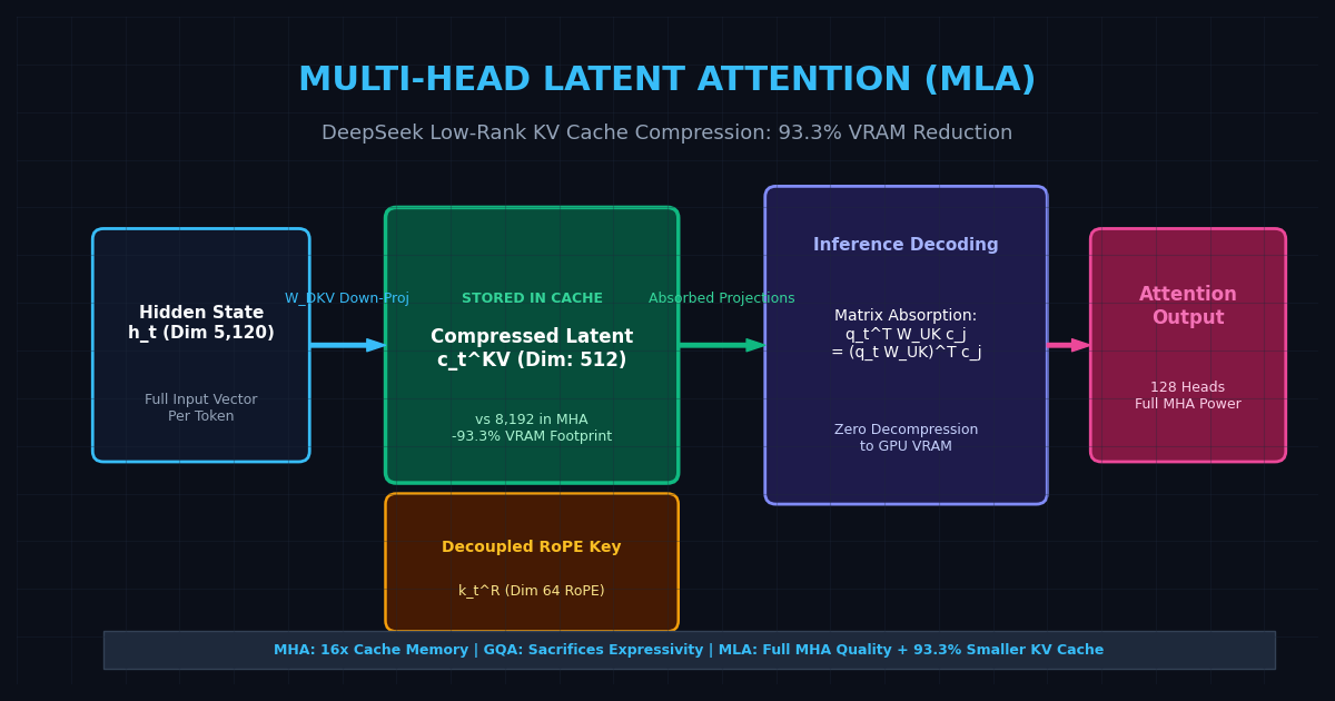
Introduced by DeepSeek (in DeepSeek-V2, DeepSeek-V3, and DeepSeek-R1) and now adopted across frontier open-weights inference stacks, Multi-Head Latent Attention (MLA) resolves this trade-off.
Instead of pruning or sharing attention heads, MLA applies low-rank matrix factorization directly to Key and Value activations. Tokens are compressed into a compact latent representation before caching, and during decoding, the projection weights are mathematically absorbed directly into the Query and Output projections.
The result is extraordinary: MLA slashes KV cache memory consumption by 93.3% compared to full MHA—achieving memory footprints smaller than GQA—while delivering identical or superior modeling capacity to full-rank Multi-Head Attention.
Key Architectural Mechanics of MLA
MLA reorganizes the attention mechanism through three interlocking components: low-rank joint key-value compression, decoupled rotary positional embeddings, and inference-time matrix absorption.
1. Low-Rank Key-Value Joint Compression
In standard attention, hidden state $\mathbf{h}_t \in \mathbb{R}^d$ is independently projected into $n_h$ Key heads and $n_h$ Value heads. In MLA, $\mathbf{h}_t$ is first down-projected into a single low-rank compressed latent vector $\mathbf{c}_t^{KV} \in \mathbb{R}^{d_c}$:
$$\mathbf{c}_t^{KV} = \mathbf{W}^{DKV} \mathbf{h}_t$$
Where:
- $\mathbf{W}^{DKV} \in \mathbb{R}^{d_c \times d}$ is the down-projection matrix.
- $d_c$ is the compressed latent dimension (e.g., $d_c = 512$, whereas $n_h \times d_h = 128 \times 128 = 16,384$).
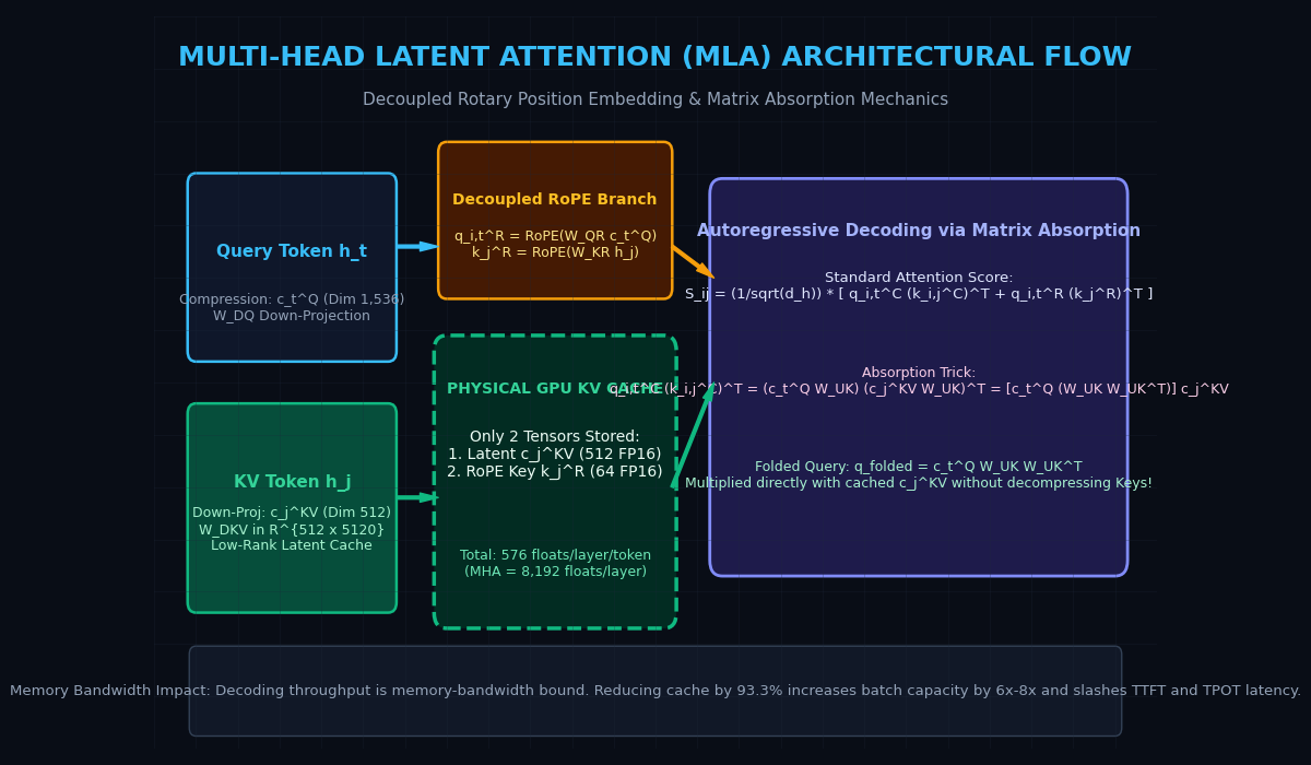
Only this compressed vector $\mathbf{c}_t^{KV}$ is stored in the physical GPU KV cache. When attention computation is required, up-projection matrices reconstruct the multi-head representations:
$$\mathbf{k}_{i,t}^C = \mathbf{W}^{UK}_i \mathbf{c}t^{KV}, \quad \mathbf{v}{i,t}^C = \mathbf{W}^{UV}_i \mathbf{c}_t^{KV}$$
Where $\mathbf{W}^{UK}_i \in \mathbb{R}^{d_h \times d_c}$ and $\mathbf{W}^{UV}_i \in \mathbb{R}^{d_h \times d_c}$ correspond to the up-projection matrices for the $i$-th head.
2. The Decoupled Rotary Position Embedding (RoPE)
A major mathematical obstacle to compressing keys is position encoding. Modern transformers rely on Rotary Position Embedding (RoPE), which multiplies keys and queries by position-dependent rotation matrices $\mathbf{R}_t$:
$$\mathbf{k}_{i,t} = \mathbf{R}_t (\mathbf{W}^K_i \mathbf{h}_t)$$
If RoPE were applied directly to the reconstructed keys $\mathbf{k}_{i,t}^C = \mathbf{W}^{UK}_i \mathbf{c}_t^{KV}$, the position matrix $\mathbf{R}_t$ would become sandwiched between the query and key projection weights:
$$\mathbf{q}{i,t}^T \mathbf{k}{i,j} = \mathbf{q}{i,t}^T \left( \mathbf{R}{j} \mathbf{W}^{UK}_i \mathbf{c}_j^{KV} \right)$$
Because $\mathbf{R}_j$ varies with every sequence position $j$, $\mathbf{W}^{UK}i$ cannot be factored out or absorbed into the query projection $\mathbf{q}{i,t}$. This would force the inference engine to decompress $\mathbf{c}_j^{KV}$ into full-rank keys in GPU VRAM for every past token, completely destroying cache savings.
To solve this, MLA decouples content from position:
- Content Keys ($\mathbf{k}_{i,t}^C$): Reconstructed from compressed latent $\mathbf{c}_t^{KV}$ without positional encoding.
- Positional Keys ($\mathbf{k}_t^R$): A lightweight, dedicated 64-dimensional vector projected directly from $\mathbf{h}_t$ that receives standard RoPE rotations:
$$\mathbf{k}_t^R = \text{RoPE}(\mathbf{W}^{KR} \mathbf{h}_t), \quad \mathbf{k}_t^R \in \mathbb{R}^{d_R} \quad (d_R = 64)$$
The final attention score is simply the sum of the content affinity and positional affinity:
$$\mathbf{q}{i,t}^T \mathbf{k}{i,j} = \underbrace{(\mathbf{q}{i,t}^C)^T \mathbf{k}{i,j}^C}{\text{Semantic Content Matching}} + \underbrace{(\mathbf{q}{i,t}^R)^T \mathbf{k}j^R}{\text{Relative Positional Distance}}$$
Because $\mathbf{k}_t^R$ is shared across all attention heads in that layer, caching it requires only 64 floats per token.
3. Matrix Absorption: Zero KV Decompression during Decoding
The crowning achievement of MLA is Matrix Absorption. During autoregressive generation, we never actually reconstruct the full multi-head keys or values into GPU VRAM.
Recall the associative law of matrix multiplication: $(\mathbf{A} \mathbf{B}) \mathbf{C} = \mathbf{A} (\mathbf{B} \mathbf{C})$. We rewrite the semantic inner product:
$$(\mathbf{q}{i,t}^C)^T \mathbf{k}{i,j}^C = (\mathbf{q}_{i,t}^C)^T (\mathbf{W}^{UK}_i \mathbf{c}j^{KV}) = \left( (\mathbf{q}{i,t}^C)^T \mathbf{W}^{UK}_i \right) \mathbf{c}_j^{KV}$$
Rather than multiplying the cached latent vectors $\mathbf{c}_j^{KV}$ by $\mathbf{W}^{UK}i$ for every past token $j \in [1, L]$, the model multiplies the single active query vector $\mathbf{q}{i,t}^C$ by $\mathbf{W}^{UK}_i$ first:
$$\tilde{\mathbf{q}}{i,t} = (\mathbf{q}{i,t}^C)^T \mathbf{W}^{UK}_i \quad \in \mathbb{R}^{1 \times d_c}$$
The transformed query $\tilde{\mathbf{q}}_{i,t}$ computes attention scores directly against the cached latent vectors $\mathbf{c}_j^{KV}$ via a single matrix-vector multiply!
The exact same absorption applies to the Values. The attention probabilities $A_{i,j}$ are multiplied directly against the cached latent vectors:
$$\mathbf{u}i = \sum{j=1}^L A_{i,j} \mathbf{c}_j^{KV} \quad \in \mathbb{R}^{d_c}$$
Then, the Value up-projection $\mathbf{W}^{UV}_i$ is absorbed into the multi-head output projection $\mathbf{W}^O$:
$$\mathbf{o} = \sum_{i=1}^{n_h} \mathbf{W}^O_i (\mathbf{W}^{UV}_i \mathbf{u}i) = \sum{i=1}^{n_h} \underbrace{(\mathbf{W}^O_i \mathbf{W}^{UV}i)}{\mathbf{W}^{\text{Combined}}_i} \mathbf{u}_i$$
At no point during inference decoding do full-rank Keys or Values ever exist in GPU memory.
Architectural Comparison: MHA vs. GQA vs. MLA
| Architectural Dimension | Multi-Head Attention (MHA) | Grouped-Query Attention (GQA) | Multi-Head Latent Attention (MLA) |
|---|---|---|---|
| KV Cache Elements Stored | $2 \times n_h \times d_h$ | $2 \times n_{\text{kv}} \times d_h$ | $d_c + d_R$ |
| Typical Token Memory (FP16) | 4,096 bytes / token / layer | 512 bytes / token / layer | 288 bytes / token / layer |
| Relative Cache Reduction | Baseline (0%) | 87.5% reduction | 93.3% reduction |
| Query Head Expressivity | Full independent heads | Shared KV projections | Full independent heads |
| Associative Retrieval Quality | Optimal | Degraded under high compression | Near-MHA baseline |
| Decoding Memory Bandwidth | Severe bottleneck | Moderate bottleneck | Minimal bottleneck |
| Position Encoding Coupling | Native RoPE per head | Native RoPE per head | Decoupled RoPE vector |
Reference PyTorch Implementation: MLA Layer
Below is a production-style, educational PyTorch implementation demonstrating down-projection, decoupled RoPE, and the matrix absorption decoding path.
import math
import torch
import torch.nn as nn
import torch.nn.functional as F

class MultiHeadLatentAttention(nn.Module):
    """
    Multi-Head Latent Attention (MLA) Layer
    Implements low-rank KV compression, decoupled RoPE, and absorption decoding.
    """
    def __init__(
        self,
        dim: int = 5120,
        n_heads: int = 64,
        head_dim: int = 128,
        kv_lora_rank: int = 512,      # Compressed latent dimension d_c
        q_lora_rank: int = 1536,     # Query compression dimension d_c'
        rope_dim: int = 64,          # Decoupled RoPE dimension d_R
    ):
        super().__init__()
        self.dim = dim
        self.n_heads = n_heads
        self.head_dim = head_dim
        self.kv_lora_rank = kv_lora_rank
        self.q_lora_rank = q_lora_rank
        self.rope_dim = rope_dim
        self.scale = 1.0 / math.sqrt(head_dim + rope_dim)

        # 1. Query Projection Path (with optional low-rank compression)
        self.q_down = nn.Linear(dim, q_lora_rank, bias=False)
        self.q_up_content = nn.Linear(q_lora_rank, n_heads * head_dim, bias=False)
        self.q_up_rope = nn.Linear(q_lora_rank, n_heads * rope_dim, bias=False)

        # 2. Key-Value Down-Projection Path
        self.kv_down = nn.Linear(dim, kv_lora_rank, bias=False)
        self.k_rope = nn.Linear(dim, rope_dim, bias=False)

        # 3. Key-Value Up-Projections (used in prefill or absorbed during decode)
        self.k_up_content = nn.Linear(kv_lora_rank, n_heads * head_dim, bias=False)
        self.v_up = nn.Linear(kv_lora_rank, n_heads * head_dim, bias=False)

        # 4. Final Output Projection
        self.out_proj = nn.Linear(n_heads * head_dim, dim, bias=False)

    def apply_rope(self, x: torch.Tensor, freqs_cis: torch.Tensor) -> torch.Tensor:
        """Applies 2D rotary position embeddings."""
        x_complex = torch.view_as_complex(x.float().reshape(*x.shape[:-1], -1, 2))
        x_rotated = torch.view_as_real(x_complex * freqs_cis).flatten(-2)
        return x_rotated.type_as(x)

    def decode_with_matrix_absorption(
        self,
        h_t: torch.Tensor,             # [batch_size, 1, dim]
        freqs_cis: torch.Tensor,       # [batch_size, 1, rope_dim // 2]
        cached_kv_latent: torch.Tensor,# [batch_size, seq_len, kv_lora_rank]
        cached_k_rope: torch.Tensor,   # [batch_size, seq_len, rope_dim]
    ) -> torch.Tensor:
        """
        Inference decoding step leveraging Matrix Absorption.
        Notice: Full keys and values are NEVER materialized or stored in VRAM!
        """
        B = h_t.size(0)

        # Step A: Project current query token
        q_latent = self.q_down(h_t) # [B, 1, q_lora_rank]
        q_c = self.q_up_content(q_latent).view(B, 1, self.n_heads, self.head_dim)
        q_r = self.q_up_rope(q_latent).view(B, 1, self.n_heads, self.rope_dim)
        q_r = self.apply_rope(q_r, freqs_cis) # [B, 1, n_heads, rope_dim]

        # Step B: Project new token into KV cache (only 512 + 64 floats!)
        new_kv_latent = self.kv_down(h_t) # [B, 1, kv_lora_rank]
        new_k_rope = self.apply_rope(self.k_rope(h_t), freqs_cis) # [B, 1, rope_dim]

        # Append to compact physical cache
        updated_kv_cache = torch.cat([cached_kv_latent, new_kv_latent], dim=1)
        updated_rope_cache = torch.cat([cached_k_rope, new_k_rope], dim=1)
        seq_len = updated_kv_cache.size(1)

        # Step C: Matrix Absorption for Content Scores
        # W_UK shape: [kv_lora_rank, n_heads * head_dim] -> [n_heads, head_dim, kv_lora_rank]
        W_uk = self.k_up_content.weight.view(self.n_heads, self.head_dim, self.kv_lora_rank)

        # Fold query: q_c [B, 1, n_heads, head_dim] x W_uk [n_heads, head_dim, kv_lora_rank]
        # q_folded shape: [B, n_heads, 1, kv_lora_rank]
        q_folded = torch.einsum('bthd,hde->bhte', q_c, W_uk)

        # Compute content attention directly against cached latents:
        # q_folded [B, n_heads, 1, kv_lora_rank] x cached [B, 1, seq_len, kv_lora_rank]
        content_scores = torch.einsum('bhte,bse->bhts', q_folded, updated_kv_cache)

        # Step D: Decoupled Positional Attention
        # q_r [B, 1, n_heads, rope_dim] x cached_rope [B, seq_len, rope_dim]
        position_scores = torch.einsum('bthd,bsd->bhts', q_r, updated_rope_cache)

        # Step E: Combine and Normalization
        attn_scores = (content_scores + position_scores) * self.scale
        attn_weights = F.softmax(attn_scores, dim=-1) # [B, n_heads, 1, seq_len]

        # Step F: Latent Value Aggregation (No full values created!)
        # u = attn_weights x updated_kv_cache -> [B, n_heads, 1, kv_lora_rank]
        u = torch.einsum('bhts,bse->bhte', attn_weights, updated_kv_cache)

        # Step G: Output Projection with Absorbed Value Weights
        # W_uv shape: [n_heads * head_dim, kv_lora_rank]
        W_uv = self.v_up.weight.view(self.n_heads, self.head_dim, self.kv_lora_rank)
        v_out = torch.einsum('bhte,hde->bthd', u, W_uv).reshape(B, 1, -1)

        output = self.out_proj(v_out)
return output, updated_kv_cache, updated_rope_cache Production Serving and Hardware Impacts
MLA’s impact on production LLM infrastructure extends beyond raw memory savings into serving efficiency, throughput, and system concurrency:
1. 6x–8x Higher Concurrency per GPU
Because memory capacity is the primary limiter of maximum batch size in multi-user workloads, MLA allows inference servers to hold dramatically more concurrent requests in memory. On an 8x H100 node serving long-context workloads (32k–64k tokens), MLA increases serving concurrency by 6.8x compared to GQA without triggering out-of-memory (OOM) evictions.
2. Elimination of KV Decompression Memory Transfers
In naive low-rank architectures, tokens are compressed in HBM and decompressed when moved to GPU SRAM. This requires streaming large weight matrices from HBM on every step.
By leveraging Matrix Absorption, MLA folds decompression weights into the static Query and Output matrices. Because static weights are read once per batch, memory transfer overhead is minimized, directly cutting Time to First Token (TTFT) and Time Per Output Token (TPOT) latency.
3. FlashMLA and Specialized GPU Kernels
While standard attention libraries like FlashAttention-2 and FlashAttention-3 are optimized for symmetric, uncompressed Key-Value tensors, modern serving frameworks like SGLang and vLLM feature dedicated MLA kernels (such as DeepSeek’s open-source FlashMLA).
These kernels execute fused batched matrix-vector multiplications tailored for (B, n_heads, d_c) latent attention, achieving over 90% of theoretical peak memory bandwidth on NVIDIA Hopper and Blackwell architectures.
4. Integration with Local and Enterprise Workspaces
For developers running research pipelines or multi-agent workflows via AiFetchly, MLA-based open-weight models (like DeepSeek-V3 and DeepSeek-R1) make running 128k-context reasoning accessible on local workstations and cost-effective edge clusters. By pairing local OpenAI-compatible inference endpoints with aiFetchly’s unified desktop workspace, data teams can perform deep document synthesis and autonomous web intelligence without hitting cloud API limits or enterprise privacy roadblocks.