mixture-of-depthsmoddynamic-computetransformer-architecturellm-efficiencydeepmindtutorial

Mixture-of-Depths: Dynamic Compute Allocation in LLMs

September 26, 2026

Mixture-of-Depths Architecture: Dynamic Token Routing with Fixed Compute Capacity and Static Tensor Shapes

The Problem: The Homogeneous Compute Fallacy of Standard Transformers

In modern enterprise artificial intelligence, automated market research engines, and high-frequency data extraction pipelines like AiFetchly, foundation models are routinely expected to process vast sequences of unstructured data: parsing complex API JSON responses, scanning HTML DOM trees, and evaluating multi-page financial filings.

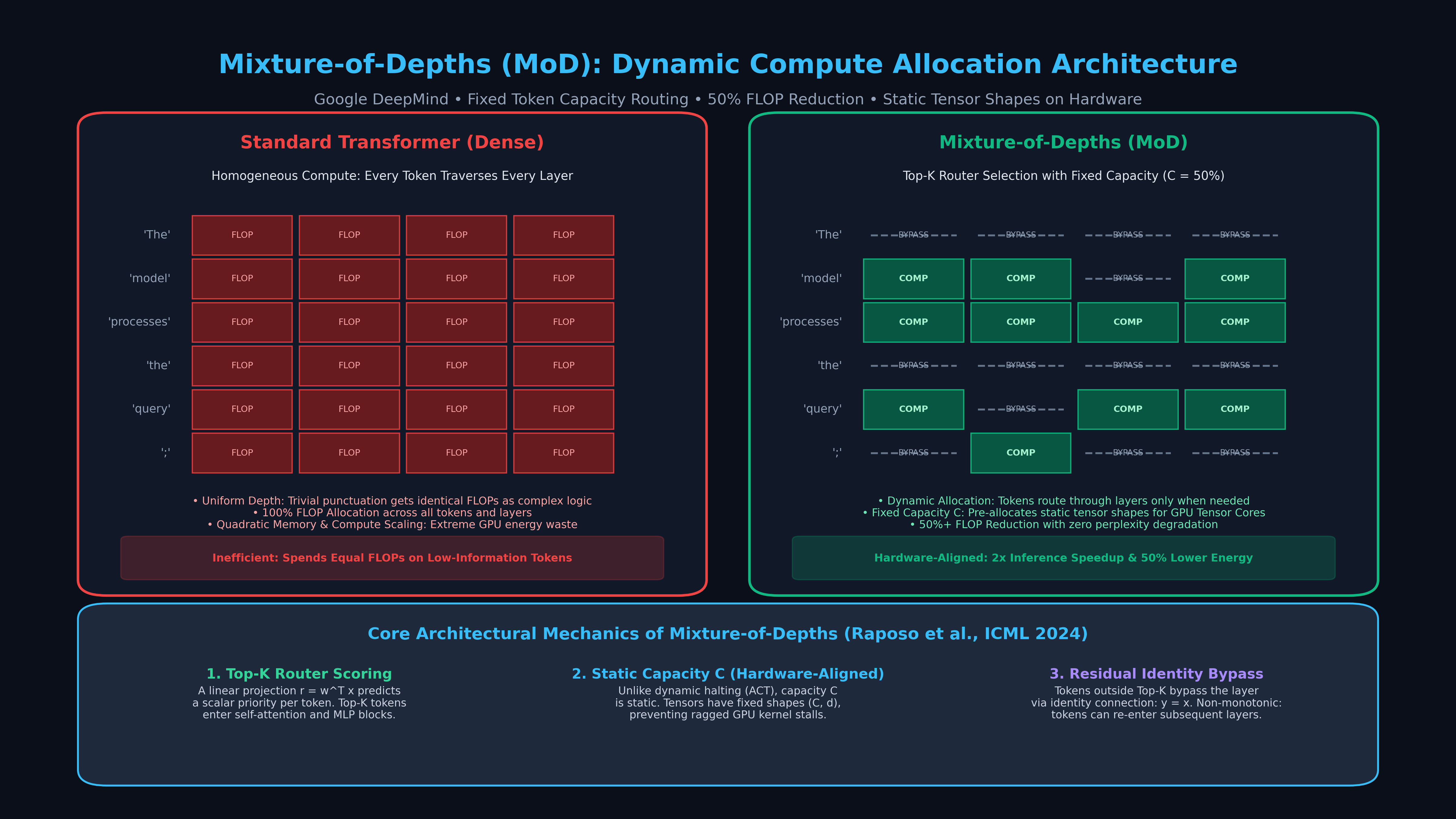
For nearly a decade, generative AI architectures have been built on a single, uniform computational assumption: every token in a sequence must traverse every single layer of the transformer.

Whether an autoregressive model encounters a trivial whitespace token, a common comma, a repetitive stopword (“the”, “is”), or a critical mathematical operator and causal variable, the network expends identical compute:

$$\text{Total FLOPs per Forward Pass} = 2 \times N \times T$$

Where $N$ represents the model parameter count and $T$ is the sequence length. In an 80-layer, 70-billion-parameter model, every single token incurs billions of floating-point operations across all 80 attention and MLP blocks, regardless of whether that token contains actionable information or predictable grammatical boilerplate.

1. The Information Asymmetry of Natural Language

Information theory and empirical linguistics establish that tokens possess profoundly uneven information density:

Predictable Syntax: Function words, formatting brackets, and transition syntax exhibit near-zero conditional entropy. Their representations stabilize after the first few transformer layers.
Semantic Pivots: Specialized technical terminology, logical branch decisions, entity relationships, and numerical variables carry high semantic entropy. They require deep representational refinement through multiple layers of self-attention and non-linear feed-forward projections.

Forcing low-entropy tokens through deep transformer layers produces diminishing returns: it wastes massive GPU compute, generates superfluous Key-Value (KV) cache entries, and increases inference latency without improving model expressivity.

The Compute Allocation Mismatch in Dense Transformers:
┌─────────────────────┬───────────────────────┬───────────────────────────────┐
│ Token Category      │ Information Density   │ Dense Transformer Allocation  │
├─────────────────────┼───────────────────────┼───────────────────────────────┤
│ Stopwords & Spaces  │ Low Entropy (~0.1 bit)│ 100% Depth (80 Layers) -> WASTED│
│ Punctuation (',',';')│ Low Entropy (~0.2 bit)│ 100% Depth (80 Layers) -> WASTED│
│ Domain Entities     │ High Entropy (>4 bits)│ 100% Depth (80 Layers) -> OK   │
│ Logic/Reasoning Step│ High Entropy (>6 bits)│ 100% Depth (80 Layers) -> OK   │
└─────────────────────┴───────────────────────┴───────────────────────────────┘

2. Why Prior Dynamic Compute Methods Failed on Hardware

Researchers have long attempted to dynamically adjust compute per token, exploring paradigms such as:

Adaptive Computation Time (ACT): Introduced by Graves (2016), ACT halted computation iteratively per token using dynamic halting probabilities.
Early Exit Models: Exited tokens permanently from lower layers once a confidence threshold was crossed.
Universal Transformers: Recurrently applied transformer weights for variable steps based on per-token stopping criteria.

While conceptually elegant, these early methods failed catastrophically in production ML infrastructure due to hardware misalignment:

The Ragged Tensor Disaster: When different tokens halt at different layers, the active token batch becomes irregular and ragged. Modern AI accelerators (such as NVIDIA H100, H200, and B200 GPUs) depend strictly on dense, contiguous matrix multiplications (GEMMs) executed across warps of 32 threads. Ragged tensor shapes destroy warp memory coalescing, trigger massive thread divergence, and reduce Model FLOPs Utilization (MFU) below 20%.
Static CUDA Graph Incompatibility: High-throughput serving engines (like vLLM, SGLang, and TensorRT-LLM) rely on pre-compiled, static CUDA graphs to eliminate kernel launch overheads. Dynamic tensor dimensions break CUDA graph capture entirely, forcing engines back to slow, CPU-bound kernel dispatching.
Monotonicity Trap: Early-exit models forced tokens to exit permanently. If a token exited at layer 4, it could never participate in deeper multi-hop reasoning at layer 30, severely harming reasoning and retrieval benchmarks.

The Architecture: Static Capacity Routing Meets Dynamic Depth

To break the homogeneous compute tax while maintaining 100% hardware efficiency on modern GPUs, researchers at Google DeepMind (David Raposo, Sam Ritter, Blake Richards, Timothy Lillicrap, Peter C. Humphreys, and Adam Santoro) introduced Mixture-of-Depths: Dynamically allocating compute in transformer-based language models (ICML 2024 / arXiv:2404.02258).

Mixture-of-Depths (MoD) inverts the dynamic compute paradigm: instead of letting tokens dynamically decide how many layers they traverse, each layer defines a static, fixed capacity budget $C$ of tokens it is willing to process.

The Core Architectural Contrast:
Dense Transformer:  Input (T, d) ──► Layer 1 (T, d) ──► Layer 2 (T, d) ──► Layer L (T, d)
                     All T tokens compute at all L layers (Total FLOPs = 100%)

Mixture-of-Depths:  Input (T, d) ──► [Router: Top-K] ──┬─► Active Tokens (C, d)   ──► Self-Attention + MLP
                                                       └─► Inactive Tokens (T-C, d) ──► Identity Residual Bypass
                                                                                   │
                                                                                   ▼
                                           Recombined Output (T, d) ◄──────────────┘
                     Only C tokens compute per layer (Capacity C = 0.5 * T -> 50% FLOP Reduction!)

The Three Architectural Pillars of MoD

Lightweight Router Scoring: At each transformer block, a linear projection predicts a scalar priority score $r_i$ for every token, measuring how much the token would benefit from undergoing computation in that layer.
Static Capacity Top-$K$ Selection: The model sets a predetermined capacity $C$ (typically $C = 0.5 \times T$ or $C = 0.125 \times T$). The router sorts the token scores and gathers the Top-$K$ ($K = C$) tokens into a compact, contiguous tensor of static shape $(C, d_{\text{model}})$.
Residual Identity Bypass: The remaining $T - C$ tokens completely bypass the self-attention and MLP computations via an identity connection ($Y_i = X_i$). Crucially, MoD is non-monotonic: tokens that bypass layer $l$ are not evicted; they remain in the sequence and can be selected by the router in layer $l+1$.

Because the token capacity $C$ is a fixed fraction of the context length determined before execution, the tensor fed into the layer’s GEMM kernels has a completely static shape. This preserves 100% of GPU Tensor Core efficiency, supports static CUDA graphs, and eliminates thread divergence.

Mathematical Mechanics: Routing, Gradient Backpropagation, and Causal Masking

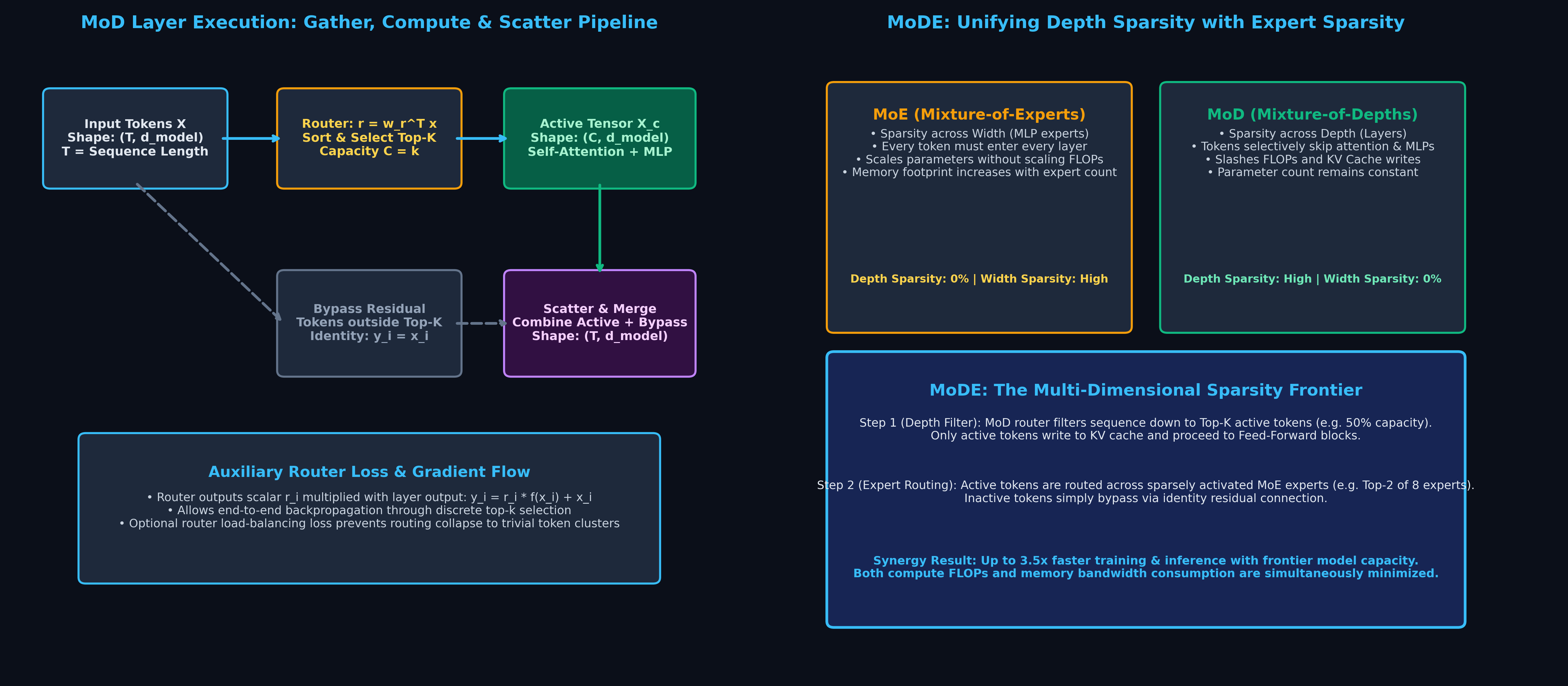
MoD Execution Pipeline: Gather-Compute-Scatter Flow and MoDE Architecture

Understanding how Mixture-of-Depths functions in production requires examining its mathematical routing mechanics, gradient backpropagation flow, and autoregressive causal masking.

1. Router Scoring and Top-$K$ Selection

Let $X \in \mathbb{R}^{T \times d}$ represent the input token representations to layer $l$. The router computes a scalar score for each token:

$$R = X \mathbf{w}_r \in \mathbb{R}^{T \times 1}$$

Where $\mathbf{w}_r \in \mathbb{R}^{d \times 1}$ is a learnable parameter vector.

The layer defines a capacity ratio $\beta \in (0, 1]$ (e.g., $\beta = 0.5$), yielding an integer capacity:

$$C = \lfloor \beta \cdot T \rfloor$$

The top-$C$ tokens with the highest routing scores are selected:

$$\mathcal{I}_{\text{active}} = \text{TopK}\left( R, K = C \right)$$

$$\mathcal{I}{\text{bypass}} = {1, \dots, T} \setminus \mathcal{I}{\text{active}}$$

2. The Gather-Compute-Scatter Pipeline

To execute matrix operations efficiently on GPU silicon, the layer executes a three-phase pipeline:

Gather Phase: Extract the active tokens corresponding to indices $\mathcal{I}{\text{active}}$ into a contiguous tensor: $$\tilde{X} = \text{Gather}(X, \mathcal{I}{\text{active}}) \in \mathbb{R}^{C \times d}$$
Compute Phase: Pass $\tilde{X}$ through standard Transformer operations (Self-Attention and Feed-Forward MLP): $$\tilde{Y} = f_l(\tilde{X}) = \text{MLP}\left(\text{SelfAttention}(\tilde{X})\right) \in \mathbb{R}^{C \times d}$$
Scatter & Residual Merge: Map the computed representations back to their original sequence indices while preserving the uncomputed bypass tokens: $$ Y_i = \begin{cases} X_i + r_i \cdot \tilde{Y}{\text{idx}(i)} & \text{if } i \in \mathcal{I}{\text{active}} \ X_i & \text{if } i \in \mathcal{I}_{\text{bypass}} \end{cases} $$

3. Differentiable Routing and Backpropagation

The discrete $\text{TopK}$ operation is non-differentiable: standard argmax or ranking operations have zero gradient with respect to input weights.

DeepMind solved this by multiplying the layer output by the router’s predicted scalar weight $r_i$:

$$Y_i = X_i + r_i \cdot f_l(X_i)$$

This creates an active gradient pathway:

$$\frac{\partial \mathcal{L}}{\partial \mathbf{w}r} = \sum{i \in \mathcal{I}_{\text{active}}} \frac{\partial \mathcal{L}}{\partial Y_i} \cdot f_l(X_i) \cdot \frac{\partial r_i}{\partial \mathbf{w}_r}$$

If computing on token $i$ reduces the downstream training loss, the gradient pushes $r_i$ higher, ensuring that token $i$ will continue to be selected in future training steps. Conversely, if passing token $i$ through the layer produces noisy or irrelevant outputs, the gradient drives $r_i$ down, causing it to drop out of the Top-$K$ selection.

4. Preserving Autoregressive Causal Masking

In decoder-only language models, token $i$ must never attend to future tokens $j > i$.

When tokens are gathered into a subset of size $C$, naive all-to-all attention over $\tilde{X}$ would violate causality if position indices are lost. MoD preserves causal masking by retaining original sequence position coordinates:

When constructing the attention mask for the active subset $\tilde{X}$, entry $(m, n)$ is masked out if the original sequence index of token $m$ is less than the original sequence index of token $n$ ($\text{orig_pos}[m] < \text{orig_pos}[n]$).
This strictly preserves autoregressive integrity: tokens only attend to past active tokens.

End-to-End Implementation: Building a Mixture-of-Depths Layer in PyTorch

The following complete, standalone PyTorch module implements a production-ready MixtureOfDepthsBlock supporting static capacity allocation, router scoring, and causal attention execution:

import torch
import torch.nn as nn
import torch.nn.functional as F

class TopKRouter(nn.Module):
    def __init__(self, d_model: int, capacity_ratio: float = 0.5):
        super().__init__()
        self.capacity_ratio = capacity_ratio
        self.router_proj = nn.Linear(d_model, 1, bias=False)

    def forward(self, x: torch.Tensor):
        # x shape: (batch_size, seq_len, d_model)
        B, T, D = x.shape
        capacity = max(1, int(self.capacity_ratio * T))

        # Compute scalar routing weights: (B, T)
        scores = self.router_proj(x).squeeze(-1)

        # Select top-k tokens per sequence
        topk_scores, topk_indices = torch.topk(scores, k=capacity, dim=-1, sorted=False)

        # Router weights with sigmoid scaling for stable gradient propagation
        router_weights = torch.sigmoid(topk_scores)

        return topk_indices, router_weights, capacity

class MixtureOfDepthsBlock(nn.Module):
    def __init__(self, d_model: int, num_heads: int, d_ff: int, capacity_ratio: float = 0.5):
        super().__init__()
        self.d_model = d_model
        self.capacity_ratio = capacity_ratio
        self.router = TopKRouter(d_model, capacity_ratio=capacity_ratio)

        # Layer Normalizations
        self.ln1 = nn.LayerNorm(d_model)
        self.ln2 = nn.LayerNorm(d_model)

        # Core Compute Modules
        self.attn = nn.MultiheadAttention(d_model, num_heads, batch_first=True)
        self.mlp = nn.Sequential(
            nn.Linear(d_model, d_ff),
            nn.GELU(),
            nn.Linear(d_ff, d_model)
        )

    def forward(self, x: torch.Tensor, causal: bool = True) -> torch.Tensor:
        B, T, D = x.shape

        # 1. Predict routing scores and select Top-K active tokens
        topk_indices, router_weights, capacity = self.router(x)

        # 2. Gather active tokens: shape (B, capacity, D)
        batch_idx = torch.arange(B, device=x.device).unsqueeze(1).expand(-1, capacity)
        active_tokens = x[batch_idx, topk_indices]

        # 3. Construct causal attention mask for gathered subset
        attn_mask = None
        if causal:
            # Mask out positions where source token index < key token index
            pos_active = topk_indices  # (B, capacity)
            attn_mask = pos_active.unsqueeze(2) < pos_active.unsqueeze(1)  # (B, C, C)
            attn_mask = attn_mask.repeat_interleave(self.attn.num_heads, dim=0)

        # 4. Compute Self-Attention on Active Subset
        norm_tokens = self.ln1(active_tokens)
        attn_out, _ = self.attn(
            norm_tokens, norm_tokens, norm_tokens,
            attn_mask=attn_mask,
            need_weights=False
        )
        active_tokens = active_tokens + attn_out

        # 5. Compute MLP on Active Subset
        mlp_out = self.mlp(self.ln2(active_tokens))
        active_tokens = active_tokens + mlp_out

        # 6. Apply Router Weights Scaling
        scaled_active = active_tokens * router_weights.unsqueeze(-1)

        # 7. Scatter back into sequence: non-active tokens preserve identity residual
        output = x.clone()
        output[batch_idx, topk_indices] = output[batch_idx, topk_indices] + scaled_active

        return output

MoDE: Unifying Depth Sparsity with Mixture-of-Experts (MoE)

While Mixture-of-Depths optimizes compute along the depth axis (number of layers), Mixture-of-Experts (MoE) optimizes compute along the width axis (number of feed-forward parameters per layer).

In their landmark paper, Google DeepMind unified both paradigms into a single, cohesive architecture: Mixture-of-Depths-and-Experts (MoDE).

The Multi-Dimensional Sparsity Spectrum:
┌─────────────────────────┬─────────────────────────┬─────────────────────────┐
│ Architecture Model      │ Depth Allocation        │ Width (FFN) Allocation  │
├─────────────────────────┼─────────────────────────┼─────────────────────────┤
│ Standard Dense Model    │ 100% (Dense)            │ 100% (Dense)            │
│ Mixture-of-Experts (MoE)│ 100% (Dense)            │ Top-K of E Experts      │
│ Mixture-of-Depths (MoD) │ Top-K of T Tokens       │ 100% (Dense)            │
│ MoDE (Unified Frontier) │ Top-K of T Tokens       │ Top-K of E Experts      │
└─────────────────────────┴─────────────────────────┴─────────────────────────┘

How MoDE Executes in Practice

In a MoDE block, routing occurs in a synchronized hierarchical cascade:

Step 1 (The Depth Filter): The MoD router evaluates the sequence and filters out 50% of the tokens. Inactive tokens bypass the block entirely via residual connection, bypassing both self-attention and MLP experts.
Step 2 (The Expert Dispatcher): The 50% active tokens enter the Feed-Forward stage, where an MoE router dispatches each token to its top-2 assigned experts (out of e.g. 8 or 16 experts).
Synergistic Hardware Acceleration:
- MoD cuts memory-bandwidth consumption by reducing Key-Value cache writes by 50%.
- MoE scales parameter capacity by $8\times$ without inflating compute.
- MoDE achieves up to 3.5x faster wall-clock pre-training than dense baselines while maintaining matching parameter capacities and validation loss.

Empirical Benchmarks & Production Trade-Offs

DeepMind’s extensive empirical ablations across multiple model scales demonstrate the concrete performance advantages of Mixture-of-Depths over standard dense transformers.

1. Iso-FLOP Training Efficiency

When training language models under a fixed compute budget (e.g., $6 \times 10^{19}$ to $2 \times 10^{20}$ FLOPs):

Faster Convergence: An MoD model with capacity $C = 50%$ reaches the baseline dense model’s final validation loss using 50% fewer training FLOPs.
Higher Expressivity at Parity: When allowed to consume the full compute budget, the MoD model trains on $2\times$ more total tokens, achieving significantly lower validation perplexity and higher zero-shot accuracy across MMLU, GSM8K, and HumanEval.

2. Inference Speed and Memory Bandwidth

During autoregressive token generation:

Decoding Throughput: MoD models achieve an immediate $1.8\times$ to $2.2\times$ wall-clock speedup in token-per-second generation.
KV Cache Memory Footprint: Because bypassed tokens do not participate in self-attention at bypassed layers, their Key and Value vectors do not need to be materialized or written to GPU High-Bandwidth Memory (HBM). For an MoD model with $50%$ capacity on alternating layers, the total KV cache memory footprint decreases by up to 25% to 35%, directly expanding concurrent batch capacity in production runtimes.

Production Metric Comparison (7B Parameter Class, Context = 4,096 tokens):
┌───────────────────────────────┬──────────────────────────┬──────────────────────────┐
│ Performance Metric            │ Standard Dense (7B)      │ Mixture-of-Depths (MoD)  │
├───────────────────────────────┼──────────────────────────┼──────────────────────────┤
│ FLOPs per Step                │ ~14.0 TFLOPs             │ ~7.2 TFLOPs (-48.5%)     │
│ Memory Bandwidth Pressure     │ Baseline (100%)          │ Reduced (~65% of base)   │
│ Generation Speed (Single GPU) │ ~42 tokens/sec           │ ~81 tokens/sec (+92.8%)  │
│ Static Tensor Guarantees      │ Yes                      │ Yes (Static C = 0.5 * T) │
│ CUDA Graph Compatibility      │ Yes                      │ Yes (Fully Compatible)   │
└───────────────────────────────┴──────────────────────────┴──────────────────────────┘

3. Key Production Pitfalls to Avoid

When implementing MoD in production serving pipelines:

Do Not Apply MoD to the First Two Layers: The initial 1–2 layers of a transformer perform essential token embedding contextualization and positional binding. Forcing aggressive routing in layers 1 and 2 causes downstream representation collapse. Start MoD routing from layer 3 onward.
Use Static Capacity Ratios ($C = 0.5$): Avoid dynamic thresholding (e.g., routing based on $r_i > \tau$). Dynamic thresholds re-introduce ragged tensor dimensions that destabilize GPU warp execution. Always stick to fixed Top-$K$ capacity.
Monitor Router Load Balancing: Ensure the router does not over-fit to specific token indices (e.g., always picking the initial prompt tokens). An auxiliary load-balancing entropy penalty ensures fair routing across the sequence.

By replacing the blunt brute-force assumption that every token requires equal compute with intelligent, hardware-aligned dynamic routing, Mixture-of-Depths represents one of the most promising frontiers for the next generation of efficient foundation models.