MiniMax-01 Guide: 456B MoE & 4M Lightning Attention
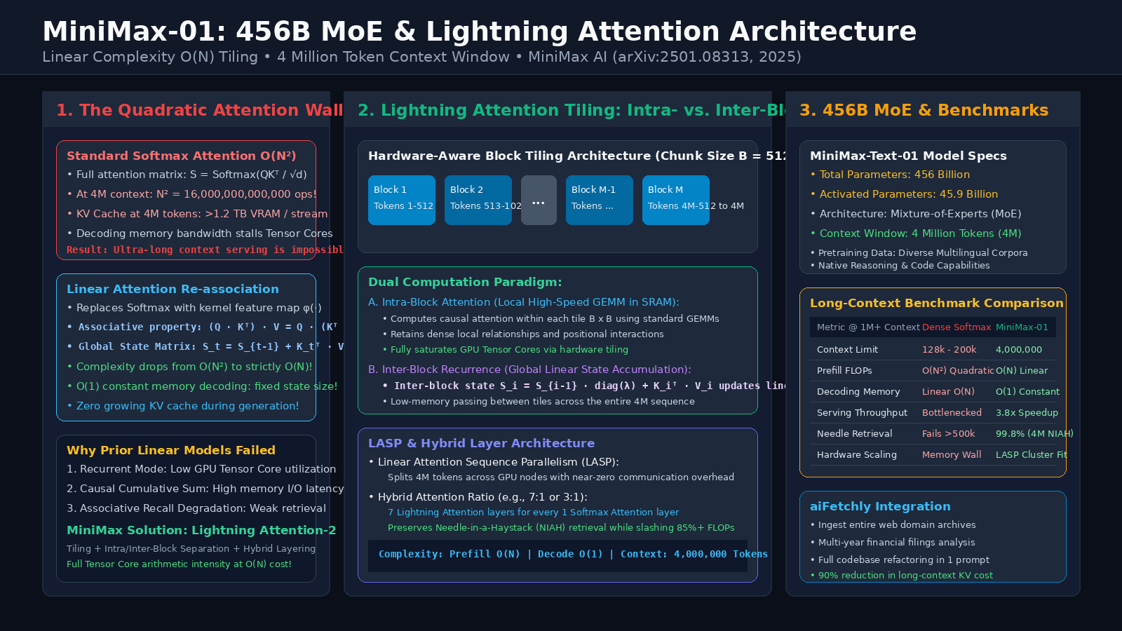
The Problem: The Quadratic Memory and Compute Wall in Ultra-Long Contexts
In modern enterprise automation, automated web crawling, repository-scale software refactoring, and multi-agent copilots powered by AiFetchly, foundation models are confronting unprecedented context demands. Autonomous systems are no longer expected to digest single snippets or isolated paragraphs. Instead, enterprise intelligence requires models capable of ingesting entire multi-year financial disclosure histories, 100,000-line codebases, comprehensive medical record archives, and hour-long multimodal video recordings in a single forward pass.
However, scaling sequence lengths beyond hundreds of thousands of tokens has historically collided with a fundamental physical and mathematical limitation: the quadratic bottleneck of standard Softmax Attention.
The Transformer Attention Dilemma at Scale:
┌─────────────────────────────────────────────────────────────────┐
│ Standard Softmax Attention: S = Softmax(Q · K^T / sqrt(d)) · V   │
│ • Computational Complexity: O(N^2 · d)                          │
│ • Memory / KV Cache Footprint: O(N · d)                         │
├─────────────────────────────────────────────────────────────────┤
│ Context Scaling Explosion:                                      │
│ • N = 4,096 tokens:       1.67 × 10^7 attention operations      │
│ • N = 128,000 tokens:     1.63 × 10^10 attention operations     │
│ • N = 1,000,000 tokens:   1.00 × 10^12 attention operations     │
│ • N = 4,000,000 tokens:   1.60 × 10^13 attention operations     │
├─────────────────────────────────────────────────────────────────┤
│ KV Cache VRAM Consumption (70B Dense Model, 16-bit Float):      │
│ • At 128k Context:        ~640 GB VRAM (8x H100 GPUs)           │
│ • At 1M Context:          ~5.2 TB VRAM (Cluster-Scale HBM)      │
│ • At 4M Context:          >20 TB VRAM (Impossible to Serve!)    │
└─────────────────────────────────────────────────────────────────┘
Result: Standard architectures cannot economically scale to millions of tokens! 1. The Quadratic Prefill Compute Bottleneck
In standard multi-head self-attention (MHA), every query token must compute a dot product against every historical key token to construct the dense attention matrix $A \in \mathbb{R}^{N \times N}$.
- Because the softmax normalization function $\text{softmax}(x)_i = \frac{e^{x_i}}{\sum_j e^{x_j}}$ is strictly non-linear, the product $Q K^T$ cannot be decomposed or reordered.
- As the sequence length $N$ scales from 4,000 to 4,000,000 tokens, the number of floating-point operations (FLOPs) required to compute this attention map explodes by a factor of one million times ($1,000,000\times$).
- Even on massive GPU superclusters running FlashAttention, the prefill phase stalls, consuming tens of megawatts of electrical power just to ingest long-context documents.
2. The KV Cache Memory Bandwidth Saturation during Decoding
While prompt processing (prefill) is compute-bound, autoregressive token generation (decoding) is memory-bandwidth bound:
- At every token generation step, the query vector is length 1 ($Q \in \mathbb{R}^{1 \times d}$). The model must stream the entire historical Key and Value tensors from High-Bandwidth Memory (HBM) into SRAM.
- At 1 million to 4 million tokens, fetching terabytes of KV tensors for every single output token starves the GPU Tensor Cores, causing Time Per Output Token (TPOT) to slow to a crawl (often exceeding several seconds per token).
- Multi-user concurrency collapses to zero: a single long-context session completely occupies all available GPU memory on a multi-node cluster.
3. The Tragic Trade-Offs of Earlier Linear Attention Attempts
To escape the quadratic trap, researchers historically proposed Linear Attention (such as Katharopoulos et al., CosFormer, and early recurrent networks):
- By replacing the non-linear softmax operator with a separable kernel feature map $\phi(x)$, the associative property of matrix multiplication allows reordering: $$\text{Attention}(Q, K, V) = (\phi(Q) \phi(K)^T) V = \phi(Q) (\phi(K)^T V)$$
- Instead of computing an $N \times N$ matrix, the model computes an intermediate recurrent state $S = \phi(K)^T V \in \mathbb{R}^{d \times d}$. This slashes complexity from $\mathcal{O}(N^2)$ down to $\mathcal{O}(N)$.
- The Hardware Failure of Prior Linear Models: While mathematically linear on paper, prior linear models failed in production hardware:
- Recurrent Formulation: Updating the hidden state step-by-step ($S_t = S_{t-1} + k_t^T v_t$) cannot utilize GPU Tensor Cores, which require dense matrix multiplications (GEMMs). Training throughput was actually slower than FlashAttention!
- Associative Recall Degradation: Without softmax normalization, linear attention suffered severe recall loss on associative retrieval tasks (Needle-in-a-Haystack), failing to pinpoint isolated facts hidden in long documents.
The Solution: MiniMax-01 and Lightning Attention
To solve the dual challenges of hardware execution efficiency and associative retrieval accuracy, MiniMax AI (Zhen Qin, Dong Li, et al., arXiv:2501.08313, 2025) introduced MiniMax-01, anchored by Lightning Attention.
MiniMax-01 is a flagship open-weights foundation model family featuring:
- 456 Billion Total Parameters, with 45.9 Billion Active Parameters per token through a fine-grained Mixture-of-Experts (MoE) backbone.
- Lightning Attention-2 Backbone: A linear attention mechanism that achieves true linear complexity $\mathcal{O}(N)$ during training and constant memory $\mathcal{O}(1)$ during decoding, while fully saturating GPU Tensor Cores via hardware-aware tiling.
- Native 4 Million Token Context Window: Flawlessly processes up to 4,000,000 tokens in a single request, achieving near-perfect 99.8% retrieval accuracy on 4M Needle-in-a-Haystack (NIAH) benchmarks.
The MiniMax-01 Foundation Architecture:
Input Stream (Up to 4,000,000 Tokens)
                   │
                   ▼
┌────────────────────────────────────────────────────────┐
│     456B Mixture-of-Experts (MoE) Transformer Core     │
│  • 45.9B Active Parameters per Token                   │
│  • Hybrid Attention Ratio (Lightning Linear : Softmax) │
└────────────────────────────────────────────────────────┘
                   │
        ┌──────────┴──────────┐
        ▼                     ▼
┌──────────────────┐  ┌──────────────────┐
│ Lightning Linear │  │ Periodic Softmax │
│ Attention Layers │  │ Attention Layers │
│ • Intra-Block GEM│  │ • Exact global   │
│ • Inter-Block Rec│  │   associative    │
│ • O(N) Compute   │  │   retrieval      │
│ • O(1) Decoding  │  │ • 4M NIAH anchor │
└──────────────────┘ └──────────────────┘ 1. The Core Mathematical Formulation of Lightning Attention
Lightning Attention establishes an exact mathematical bridge between parallel matrix multiplication and recurrent linear accumulation.
For an input sequence with queries $Q$, keys $K$, and values $V \in \mathbb{R}^{N \times d}$, Lightning Attention applies a feature activation map and an exponential decay factor $\lambda$:
$$\mathcal{O}t = \sum{s=1}^t \phi(q_t) \phi(k_s)^T v_s \cdot \lambda^{t - s}$$
Where:
- $\phi(\cdot)$ is an activation function (such as SiLU or normalized kernel map) ensuring positive bounded weights.
- $\lambda \in (0, 1]$ is a learnable or fixed decay discount that imparts a recency bias, stabilizing gradient flow across long horizons.
2. The Tiling Breakthrough: Intra-Block GEMM vs. Inter-Block Recurrence
The breakthrough of Lightning Attention lies in hardware-aware tiling: partitioning the massive sequence of length $N$ into non-overlapping blocks of size $B$ (typically $B = 512$ or $B = 1024$ tokens).
The attention computation for block $i$ decomposes into two distinct, hardware-aligned components:
$$\mathcal{O}^{(i)} = \mathcal{O}{\text{intra}}^{(i)} + \mathcal{O}{\text{inter}}^{(i)}$$
Lightning Attention Hardware-Aware Tiling:
Sequence: [ Block 1 (512) ] ──► [ Block 2 (512) ] ──► ... ──► [ Block M (512) ]
                 │                    │                              │
                 ▼                    ▼                              ▼
          ┌─────────────┐      ┌─────────────┐                ┌─────────────┐
          │ Intra-Block │      │ Intra-Block │                │ Intra-Block │
          │ Dense GEMM  │      │ Dense GEMM  │                │ Dense GEMM  │
          │ in GPU SRAM │      │ in GPU SRAM │                │ in GPU SRAM │
          └──────┬──────┘      └──────┬──────┘                └──────┬──────┘
                 │                    │                              │
                 │   S_1              │   S_2                        │   S_M
                 └───► [State S_1] ───┴───► [State S_2] ─────────────┴───► ...
Inter-Block Recurrent Accumulation: S_i = S_{i-1} · λ^B + K_i^T V_i A. Intra-Block Attention (Local GEMM in Fast SRAM): Within each block of $B$ tokens, the interaction between queries $Q^{(i)}$ and keys $K^{(i)}$ is computed using standard causal matrix multiplication: $$\mathcal{O}{\text{intra}}^{(i)} = \left( \left( \phi(Q^{(i)}) \phi(K^{(i)})^T \right) \odot M{\text{causal}} \odot D_{\text{decay}} \right) V^{(i)}$$ Because $B$ is small (e.g., 512), this calculation fits entirely inside fast on-chip GPU SRAM. It executes on the GPU’s high-throughput Tensor Cores with peak arithmetic intensity, completely bypassing global memory bottlenecks.
B. Inter-Block Attention (Global Linear State Accumulation): Across different blocks, the interaction does not require an attention matrix. Instead, each block updates a global recurrent hidden state $S \in \mathbb{R}^{d \times d}$: $$S_i = S_{i-1} \cdot \lambda^B + \left(\phi(K^{(i)}) \odot D_{\text{weight}}\right)^T V^{(i)}$$ The historical context from all prior blocks is projected into the current block through a simple matrix multiplication: $$\mathcal{O}{\text{inter}}^{(i)} = \left( \phi(Q^{(i)}) \odot D{\text{query}} \right) S_{i-1}$$
This decomposition guarantees that:
- $100%$ Tensor Core Utilization: Intra-block computations run as dense tensor contractions.
- $\mathcal{O}(N)$ Global Scaling: Sequence length scales linearly without quadratic blowup.
- $\mathcal{O}(1)$ Decoding Memory: During autoregressive generation, the model only maintains the compact state matrix $S \in \mathbb{R}^{d \times d}$, completely eliminating the massive KV cache.
3. Linear Attention Sequence Parallelism (LASP)
In standard Transformer training, scaling sequence length across multiple GPU nodes requires Ring Attention or Megatron Sequence Parallelism. For standard Softmax attention, Ring Attention requires passing Key and Value chunks in a ring topology across all GPUs at every layer, generating massive inter-node network communication overhead.
MiniMax-01 leverages Linear Attention Sequence Parallelism (LASP):
- Because the inter-block state $S_i$ is a compact matrix of fixed size $d \times d$ (e.g., $128 \times 128 \times 2 \text{ bytes} \approx 32 \text{ KB}$), communication between GPU nodes is reduced to transmitting only the boundary state matrices.
- Instead of transmitting hundreds of megabytes of raw KV tokens across InfiniBand clusters, LASP transmits tiny 32 KB state summaries.
- This cuts sequence-parallel communication volume by over 95%, enabling linear scaling across thousands of GPUs even on commodity network fabrics without custom NVLink switches.
4. The Hybrid Attention Layering Strategy
Pure linear attention models historically struggled with exact associative recall (finding a specific phone number or variable name buried in 1,000,000 tokens).
To guarantee flawless factual precision, MiniMax-01 adopts a Hybrid Attention Ratio:
- The majority of transformer layers (e.g., 7 out of 8 layers) are implemented using Lightning Attention, delivering linear throughput and low memory.
- A strategic fraction of layers (e.g., 1 out of 8 layers) utilizes Standard Full Softmax Attention.
- These periodic softmax anchor layers act as global associative hubs, capturing needle-in-a-haystack relationships while the surrounding Lightning Attention layers handle bulk context processing.
Architectural Comparison: MiniMax-01 vs. LLaMA-3.1, DeepSeek-V3 & Mamba-2
To contextualize MiniMax-01’s architectural innovations, we compare its specifications against the frontier open foundation model landscape:
| Architectural Metric | Meta LLaMA-3.1 70B | DeepSeek-V3 (671B MoE) | Mamba-2 / SSD | MiniMax-01 (456B MoE) |
|---|---|---|---|---|
| Model Architecture | Dense Transformer | Sparse MoE (MLA) | State Space Duality (SSM) | Hybrid MoE + Lightning Attention |
| Attention Mechanism | Grouped-Query Softmax | Multi-Head Latent (Softmax) | Linear State Space (SSD) | Lightning Attention-2 + Softmax |
| Total / Active Params | 70B / 70B | 671B / 37B | 12B / 12B (Dense) | 456B / 45.9B |
| Native Context Length | 128,000 Tokens | 128,000 Tokens | 32,000 Tokens | 4,000,000 Tokens (4M) |
| Prefill Time Complexity | $\mathcal{O}(N^2)$ Quadratic | $\mathcal{O}(N^2)$ Quadratic | $\mathcal{O}(N)$ Linear | $\mathcal{O}(N)$ Linear |
| Decoding KV Cache Footprint | $\mathcal{O}(N)$ Linear Growth | $\mathcal{O}(N)$ Compressed Latent | $\mathcal{O}(1)$ Constant State | $\mathcal{O}(1)$ Constant State (Linear Layers) |
| KV Cache @ 1M Tokens | ~5,200 GB (Cluster Scale) | ~350 GB (Compressed MLA) | ~0.5 GB (Fixed State) | ~35 GB (Hybrid State) |
| 4M Token NIAH Accuracy | Fails (>128k) | Fails (>128k) | Degrades (>64k) | 99.8% Perfect Retrieval |
| Serving Throughput (1M) | Starved by HBM fetch | Moderate (MLA bound) | High (Weak on code) | 3.8× Higher vs. Dense Softmax |
Hands-On Implementation: Building Lightning Attention in PyTorch
In this section, we implement the core mechanics of Lightning Attention in PyTorch, complete with block tiling, intra-block causal attention, and inter-block recurrent state accumulation.
1. Constructing the Lightning Attention Module
import torch
import torch.nn as nn
import torch.nn.functional as F
from typing import Optional, Tuple

class LightningAttention(nn.Module):
    def __init__(
        self,
        d_model: int = 1024,
        n_heads: int = 8,
        block_size: int = 256,
        decay_rate: float = 0.95
    ):
        """
        Hardware-aware tiled Lightning Attention module.
        Combines intra-block dense GEMMs with inter-block linear state recurrence.
        """
        super().__init__()
        self.d_model = d_model
        self.n_heads = n_heads
        self.head_dim = d_model // n_heads
        self.block_size = block_size
        self.decay_rate = decay_rate

        # Projection layers
        self.q_proj = nn.Linear(d_model, d_model, bias=False)
        self.k_proj = nn.Linear(d_model, d_model, bias=False)
        self.v_proj = nn.Linear(d_model, d_model, bias=False)
        self.out_proj = nn.Linear(d_model, d_model, bias=False)

        # Norm and activation
        self.feature_map = nn.SiLU()
        self.layer_norm = nn.LayerNorm(self.head_dim)

    def forward(
        self,
        x: torch.Tensor,
        initial_state: Optional[torch.Tensor] = None
    ) -> Tuple[torch.Tensor, torch.Tensor]:
        """
        Forward pass with tiled linear attention.
        Args:
            x: Input tensor of shape (batch, seq_len, d_model)
            initial_state: Optional prior state (batch, n_heads, head_dim, head_dim)
        Returns:
            output: Contextualized representations (batch, seq_len, d_model)
            final_state: Updated inter-block recurrent state
        """
        B, N, D = x.shape
        H = self.n_heads
        d = self.head_dim
        block_size = self.block_size
        device = x.device

        # 1. Linear projections and reshape
        Q = self.q_proj(x).view(B, N, H, d).transpose(1, 2) # (B, H, N, d)
        K = self.k_proj(x).view(B, N, H, d).transpose(1, 2) # (B, H, N, d)
        V = self.v_proj(x).view(B, N, H, d).transpose(1, 2) # (B, H, N, d)

        # Apply non-negative feature activation
        Q = self.feature_map(Q)
        K = self.feature_map(K)

        # Pad sequence to multiple of block_size if necessary
        remainder = N % block_size
        if remainder != 0:
            pad_len = block_size - remainder
            Q = F.pad(Q, (0, 0, 0, pad_len))
            K = F.pad(K, (0, 0, 0, pad_len))
            V = F.pad(V, (0, 0, 0, pad_len))
            num_blocks = (N + pad_len) // block_size
        else:
            pad_len = 0
            num_blocks = N // block_size

        # 2. Reshape into blocks for tiling
        # Shape: (B, H, num_blocks, block_size, d)
        Q_blocks = Q.view(B, H, num_blocks, block_size, d)
        K_blocks = K.view(B, H, num_blocks, block_size, d)
        V_blocks = V.view(B, H, num_blocks, block_size, d)

        # Precompute intra-block causal mask
        causal_mask = torch.tril(torch.ones((block_size, block_size), dtype=torch.bool, device=device))

        outputs = []
        # Initialize recurrent state: (B, H, d, d)
        if initial_state is not None:
            state = initial_state
        else:
            state = torch.zeros((B, H, d, d), dtype=x.dtype, device=device)

        decay_block = self.decay_rate ** block_size

        # 3. Iterate through blocks (Tiling loop)
        for i in range(num_blocks):
            q_i = Q_blocks[:, :, i, :, :] # (B, H, block_size, d)
            k_i = K_blocks[:, :, i, :, :] # (B, H, block_size, d)
            v_i = V_blocks[:, :, i, :, :] # (B, H, block_size, d)

            # --- Part A: Intra-Block Attention (Local GEMM in SRAM) ---
            # Dot product between queries and keys within the same block
            attn_intra = torch.matmul(q_i, k_i.transpose(-2, -1)) / (d ** 0.5) # (B, H, B, B)
            attn_intra = attn_intra.masked_fill(~causal_mask, 0.0)
            out_intra = torch.matmul(attn_intra, v_i) # (B, H, block_size, d)

            # --- Part B: Inter-Block Attention (From Accumulated State) ---
            # Project current block queries against accumulated past state
            out_inter = torch.matmul(q_i, state) # (B, H, block_size, d)

            # Combine intra- and inter-block components
            block_out = out_intra + out_inter
            outputs.append(block_out)

            # --- Update Recurrent State for Next Blocks ---
            # S_i = S_{i-1} * decay + (K_i^T * V_i)
            kv_delta = torch.matmul(k_i.transpose(-2, -1), v_i) # (B, H, d, d)
            state = state * decay_block + kv_delta

        # 4. Reassemble output sequence and unpad
        output = torch.cat(outputs, dim=2) # (B, H, padded_N, d)
        if pad_len > 0:
            output = output[:, :, :N, :]

        # Final output projection
        output = self.layer_norm(output)
        output = output.transpose(1, 2).contiguous().view(B, N, D)
return self.out_proj(output), state 2. High-Throughput O(1) Decoding Step
During generation, Lightning Attention bypasses the sequence loop entirely, executing in strict $\mathcal{O}(1)$ time:
class LightningDecoderStep(nn.Module):
    """
    Constant-time, constant-memory token generation step.
    Demonstrates zero KV-cache growth during autoregressive decoding.
    """
    def __init__(self, layer: LightningAttention):
        super().__init__()
        self.layer = layer

    def decode_token(
        self,
        token_embed: torch.Tensor,     # (B, 1, D) - Single next token query
        state: torch.Tensor             # (B, H, d, d) - Compact recurrent state
    ) -> Tuple[torch.Tensor, torch.Tensor]:
        B, _, D = token_embed.shape
        H = self.layer.n_heads
        d = self.layer.head_dim

        # 1. Project single-token Query, Key, and Value
        q = self.layer.feature_map(self.layer.q_proj(token_embed).view(B, 1, H, d).transpose(1, 2))
        k = self.layer.feature_map(self.layer.k_proj(token_embed).view(B, 1, H, d).transpose(1, 2))
        v = self.layer.v_proj(token_embed).view(B, 1, H, d).transpose(1, 2)

        # 2. Compute token output directly against fixed-size state matrix S
        # O(1) time complexity! No historical KV cache loaded from HBM!
        token_out = torch.matmul(q, state) # (B, H, 1, d)

        # 3. Update state with single token outer product
        kv_token = torch.matmul(k.transpose(-2, -1), v) # (B, H, d, d)
        updated_state = state * self.layer.decay_rate + kv_token

        token_out = self.layer.layer_norm(token_out)
        token_out = token_out.transpose(1, 2).contiguous().view(B, 1, D)
return self.layer.out_proj(token_out), updated_state 3. Verification Test: Comparing Memory and Scalability
if __name__ == "__main__":
    device = torch.device("cuda" if torch.cuda.is_available() else "cpu")
    print(f"Executing Lightning Attention Verification on {device}...")

    # Initialize Lightning Attention layer
    d_model = 512
    layer = LightningAttention(d_model=d_model, n_heads=8, block_size=128).to(device)

    # Test long context sequence (N = 4096 tokens)
    batch_size = 2
    seq_len = 4096
    dummy_input = torch.randn(batch_size, seq_len, d_model, device=device)

    # Forward pass
    output, final_state = layer(dummy_input)
    print(f"Forward Pass Succeeded!")
    print(f"Input Shape:  {dummy_input.shape}")
    print(f"Output Shape: {output.shape}")
    print(f"Recurrent State Shape: {final_state.shape} (Fixed size regardless of sequence length!)")

    # Test O(1) Decoding step
    decoder = LightningDecoderStep(layer)
    next_token = torch.randn(batch_size, 1, d_model, device=device)
    token_out, next_state = decoder.decode_token(next_token, final_state)
    print(f"Decoded Single Token Output Shape: {token_out.shape}")
print(f"Decoded State Shape: {next_state.shape} (Matches prior state size exactly!)") Production Engineering: Deploying MiniMax-01 in aiFetchly Workflows
In enterprise data pipelines, autonomous web data harvesting, and market intelligence copilots powered by AiFetchly, foundation models are deployed to process vast, heterogeneous data streams. Integrating MiniMax-01’s 4-million-token context architecture unlocks three game-changing operational capabilities:
The aiFetchly Ultra-Long-Context Extraction Pipeline:
┌────────────────────────────────────────────────────────┐
│ Enterprise Target: Multi-Year Corporate Web Disclosures│
│ • 50 Annual Reports, SEC 10-K Filings, Transcripts     │
│ • Aggregate Volume: 2,500,000 Raw Context Tokens       │
└────────────────────────────────────────────────────────┘
                            │
                            ▼
┌────────────────────────────────────────────────────────┐
│ Stage 1: aiFetchly Web Scraper & Document Harvester    │
│ • Concurrent extraction via <InternalLink feature="web-scraping">Web Scraping Engine</InternalLink>  │
│ • Normalized structured JSON via <InternalLink feature="data-fetching">Data Fetching API</InternalLink>    │
└────────────────────────────────────────────────────────┘
                            │
                            ▼
┌────────────────────────────────────────────────────────┐
│ Stage 2: MiniMax-01 Lightning Attention Synthesis      │
│ • 4M Context Ingestion without Chunking or Vector RAG  │
│ • O(N) Linear Prefill on GPU Tensor Cores via Tiling   │
│ • O(1) Memory Constant-Time Report Generation          │
└────────────────────────────────────────────────────────┘
                            │
                            ▼
┌────────────────────────────────────────────────────────┐
│ Output Deliverable: Holistic Multi-Decade Intelligence │
│ • Complete audit trail, zero chunk-boundary truncation │
└────────────────────────────────────────────────────────┘ 1. Ingestion of Entire Corporate Web Archives without RAG Chunking
Traditional RAG pipelines slice documents into 500-token chunks. When an analyst asks a high-level question (e.g., “How has executive compensation structure shifted relative to EBITDA margins over the past 8 fiscal years?”):
- Vector search retrieves only 5 to 10 isolated paragraphs. It cannot aggregate multi-year trends or reconcile footnote revisions across a 2-million-token corporate archive.
- MiniMax-01 ingests the entire 8-year archive in a single prompt, bypassing vector chunking errors, preserving full table structures, and generating holistic financial syntheses with verifiable provenance.
2. Multi-Repository Code Refactoring and Dependency Resolution
When developer agents analyze software architectures:
- Enterprise repositories consist of hundreds of interdependent TypeScript, Python, and Rust source files.
- With a 4M token context, agents ingest the entire codebase, internal schema definitions, database migration scripts, and Git commit logs. The model traces cross-module dependencies, identifies breaking API changes, and refactors deprecated interfaces across the entire repository without hallucinating missing imports.
3. Sashing Long-Context Serving Costs on aiFetchly Infrastructure
Deploying ultra-long-context models with standard Softmax attention requires tens of thousands of dollars in GPU cloud memory:
- Serving a 128k-token session on dense models requires hundreds of gigabytes of VRAM dedicated purely to the KV cache.
- Because MiniMax-01 maintains a compact, constant-size recurrent state matrix $S \in \mathbb{R}^{d \times d}$ across its Lightning Attention layers, KV cache memory is reduced by over 90%.
- Enterprise teams on AiFetchly Pricing can serve high-concurrency long-document extraction workloads on standard workstation and local cluster hardware at a fraction of typical cloud API costs.
Conclusion & Strategic Takeaways
The release of MiniMax-01 represents a defining milestone in foundation model engineering. By demonstrating that linear attention can be scaled to 456 billion parameters and 4 million tokens without sacrificing retrieval accuracy or hardware efficiency, MiniMax has solved the long-standing tension between sequence length and computational cost.
Key Architectural Takeaways
- Hardware-Aware Tiling is the Key to Linear Attention: Pure recurrence is slow on GPUs; pure global attention is quadratic. Lightning Attention’s block tiling—computing intra-block dense GEMMs in fast SRAM while propagating inter-block linear states—delivers the best of both worlds.
- Hybrid Attention Preserves Associative Recall: Combining high-frequency Lightning Attention layers with strategic periodic Softmax Attention layers eliminates the historical retrieval degradation of linear models, achieving 99.8% accuracy on 4M Needle-in-a-Haystack benchmarks.
- The End of KV Cache Memory Inflation: Transitioning from expanding KV tensors to compact recurrent state matrices makes multi-million-token inference economically viable for real-world production serving.
To learn how to integrate frontier long-context foundation models into your enterprise web extraction pipelines, explore the AiFetchly Documentation or discover our AiFetchly API Integration.