medusaspeculative-decodingllm-inferencetree-attentiontutorial

Medusa Explained: Multi-Head Speculative Decoding Guide

September 21, 2026

Medusa Architecture: Multi-Head Speculative Prediction, Tree Attention Verification, and Draft-Model-Free Inference Acceleration

The Problem: The Memory-Bandwidth Bottleneck and Draft-Model Friction

In high-throughput enterprise pipelines and interactive AI applications like AiFetchly, generative serving is severely throttled by a fundamental hardware constraint: the memory-bandwidth bound nature of autoregressive decoding.

1. The Single-Token Generation Bottleneck

During standard autoregressive generation, a Large Language Model (LLM) generates tokens sequentially, one by one. For each token:

The entire model parameter set (e.g., 70 billion parameters, consuming ~140 GB in FP16 or ~35 GB in 4-bit) must be read from High Bandwidth Memory (HBM) into GPU Static RAM (SRAM) and Tensor Cores.
Because the arithmetic intensity of single-token generation is near $1.0 \text{ FLOP/byte}$, modern GPU Tensor Cores sit idle for over 90% of execution time, stalled while waiting for memory transfers over the memory bus.

2. The Operational Dilemma of Draft-Model Speculative Decoding

To increase arithmetic intensity, traditional Speculative Decoding (Leviathan et al., Chen et al.) pairs the primary large target model (e.g., LLaMA-3-70B) with a smaller, faster draft model (e.g., LLaMA-3-8B). The draft model speculates $K$ tokens, which the target model verifies in a single forward pass.

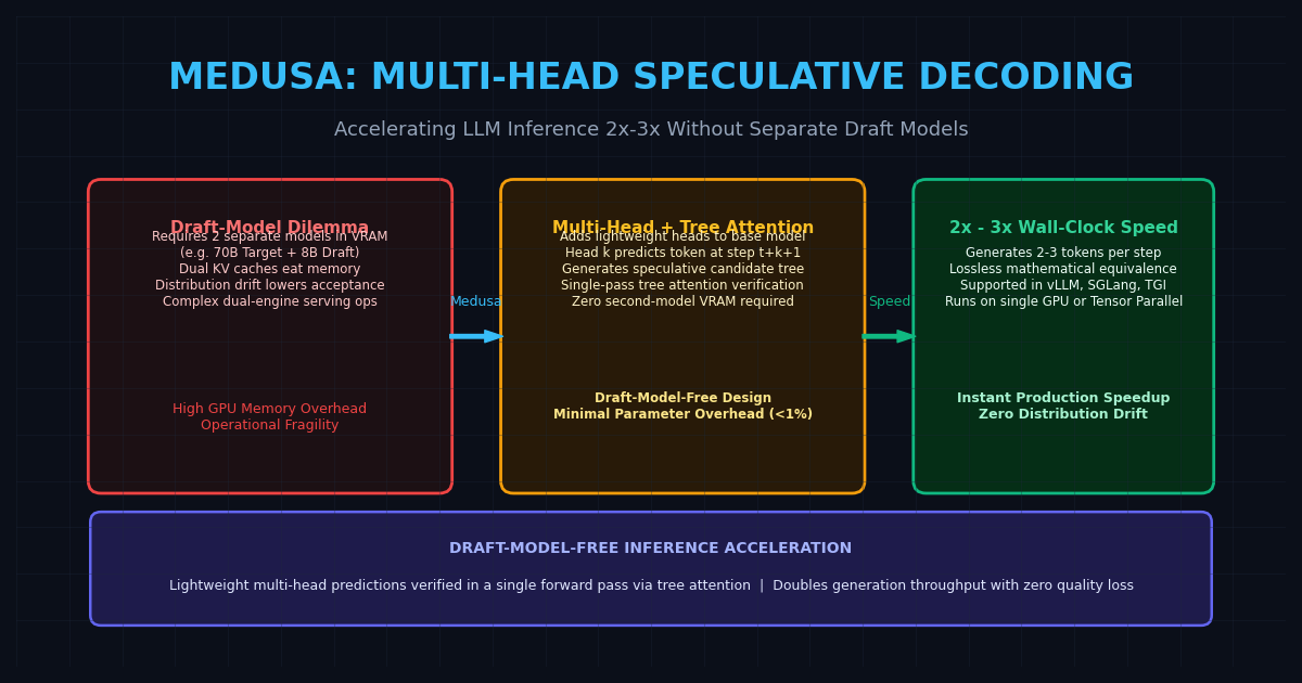
While effective in research settings, deploying dual-model speculative decoding in production creates severe operational friction:

Dual VRAM Allocation: Storing the draft model’s weights and separate Key-Value (KV) cache consumes 16 GB to 24 GB of precious GPU memory, reducing batch size and concurrency on 80 GB GPUs.
Distribution Drift: If the draft model was trained on different corpora or fine-tuned with different system prompts, its token predictions diverge from the target model. The acceptance rate $\alpha$ plummets below 40%, causing speculative decoding to run slower than baseline autoregression.
Tensor Parallelism Inefficiency: On multi-GPU clusters running 8-way Tensor Parallelism (TP=8), running a tiny 8B draft model across 8 GPUs yields disastrous latency: the computation is so light that inter-GPU NVLink All-Reduce communication dominates the execution time.
Serving Complexity: Inference engines must schedule, synchronize, and balance two distinct model graphs across heterogeneous hardware.

Production serving requires speculative acceleration without the burden of a secondary draft model.

The Solution: Medusa Multi-Head Decoding Architecture

Introduced by researchers from UIUC, Together AI, CMU, and Princeton (Tianle Cai et al., ICML 2024 / 2025), Medusa eliminates the auxiliary draft model entirely.

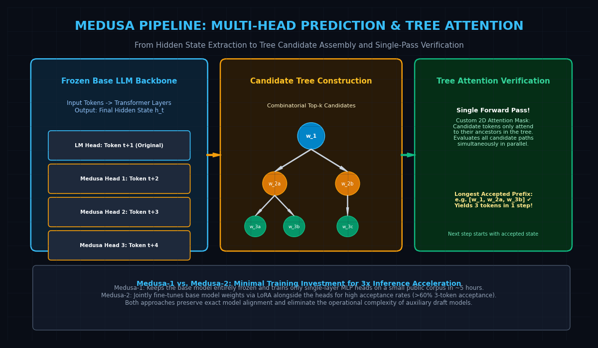
Instead of running a separate neural network, Medusa equips the base foundation model itself with multiple lightweight Medusa Heads attached directly to its final hidden layer.

Medusa Pipeline: From Hidden State Extraction to Tree Candidate Assembly and Single-Pass Verification

The Architectural Blueprint

Consider a foundation model processing input tokens up to step $t$. The final Transformer layer produces the contextual hidden state vector $\mathbf{h}_t \in \mathbb{R}^d$.

Standard autoregressive models pass $\mathbf{h}t$ through a single Language Model (LM) head to predict the immediate next token $w{t+1}$. Medusa augments this with $K$ parallel single-layer decoding heads:

Head 0 (Original LM Head): Predicts token $w_{t+1}$
Medusa Head 1: Predicts token $w_{t+2}$
Medusa Head 2: Predicts token $w_{t+3}$
Medusa Head $k$: Predicts token $w_{t+k+1}$

Each Medusa head consists of a single residual block followed by a linear projection to vocabulary dimension $V$:

$$\mathbf{h}t^{(k)} = \text{SiLU}\left(\mathbf{W}{\text{res}}^{(k)} \mathbf{h}_t\right) + \mathbf{h}t$$ $$p^{(k)}(w{t+k+1} \mid \mathbf{h}t) = \text{softmax}\left(\mathbf{W}{\text{head}}^{(k)} \mathbf{h}_t^{(k)}\right)$$

Because Medusa heads are lightweight feed-forward layers:

They add less than 1% to total parameter count (e.g., adding ~300M parameters to a 70B model).
They require zero auxiliary KV cache allocation.
They share the exact same weights, tokenizer, and tensor-parallel distribution as the base model.

Key Mechanics: Tree Candidate Construction and Tree Attention

A naive approach to multi-head prediction is greedy chaining: take the top-1 prediction from Head 1, top-1 from Head 2, etc. However, if Head 1’s single prediction is rejected by the target model, all subsequent predictions ($t+3, t+4$) are immediately invalid.

Medusa resolves this through Combinatorial Tree Candidates and Tree Attention Verification.

1. Combinatorial Tree Construction

Instead of a single linear chain, each Medusa head outputs its top-$s_k$ highest-probability tokens. Medusa combines these tokens into a Tree of Speculative Candidates:

For example, configuring top-2 for Head 1, top-2 for Head 2, and top-1 for Head 3 produces a tree of diverse candidate branches:

        Root (w_t+1)
        /          \
    w_t+2(A)     w_t+2(B)
     /    \          |
w_t+3(A1) w_t+3(A2) w_t+3(B1)
    |         |        |
w_t+4(A1) w_t+4(A2) w_t+4(B1)

By exploring multiple alternative paths in parallel, Medusa drastically increases the probability that at least one deep branch is accepted.

2. Single-Pass Tree Attention Verification

Verifying dozens of candidate branches sequentially would eliminate all latency gains. Medusa solves this by flattening the entire candidate tree into a single packed sequence and verifying it in one forward pass of the base model using Tree Attention.

Standard attention allows every token to attend to all preceding tokens in the sequence. In Tree Attention, a custom 2D attention mask $\mathbf{M}_{\text{tree}}$ ensures each candidate token attends only to its direct ancestors in the tree (plus the historical prefix context):

$$\mathbf{M}_{\text{tree}}[i, j] = \begin{cases} 0 & \text{if candidate } j \text{ is an ancestor of candidate } i \ -\infty & \text{otherwise} \end{cases}$$

Tree Attention Mask Example (5 Candidates):
       [w1] [w2a] [w2b] [w3a] [w3b]
[w1]  [  0    -inf  -inf  -inf  -inf ]
[w2a] [  0     0    -inf  -inf  -inf ]
[w2b] [  0    -inf   0    -inf  -inf ]
[w3a] [  0     0    -inf   0    -inf ]  <-- w3a attends to w1 and w2a only
[w3b] [  0    -inf   0    -inf   0   ]  <-- w3b attends to w1 and w2b only

During the single forward pass:

The base model computes attention across the packed tree in parallel.
The model outputs ground-truth probability distributions for each candidate node.
The verification algorithm finds the longest accepted path where every candidate token matches the target model’s greedy prediction.
If a 3-token branch is accepted, the model generates 3 tokens in the time of a single forward pass, achieving up to 3x wall-clock acceleration.

3. Training Paradigms: Medusa-1 vs. Medusa-2

Training Recipe	Base Model Weights	Training Compute	Data Requirement	Acceptance Rate
Medusa-1	Completely Frozen	~5 GPU hours (A100)	Small corpus (~10k ShareGPT)	High (~2.2 - 2.8 tokens/step)
Medusa-2	Fine-tuned via LoRA	~15–20 GPU hours	Public instruction dataset	Superior (~2.8 - 3.5 tokens/step)

In Medusa-1, the base model parameters remain entirely untouched; only the newly attached heads are trained via standard cross-entropy loss against shifted targets. In Medusa-2, the base model’s final layers are fine-tuned via LoRA alongside the heads, producing richer representations that push multi-token acceptance rates above 60%.

Inference Acceleration Paradigm Comparison

Feature Dimension	Standard Autoregression	Draft-Model Speculative Decoding	Lookahead Decoding	Medusa (Multi-Head)
Drafting Mechanism	None	Separate Smaller LLM (e.g. 8B)	Jacobi Fixed-Point Iteration	Parallel Medusa Heads
GPU Memory Overhead	Baseline (1x)	High (+15% to +30% for draft VRAM)	Minimal	Near Zero (<1% parameter growth)
Verification Strategy	1 token / step	Linear rejection sampling	Multi-token n-gram verification	Tree Attention (Single Forward Pass)
Distribution Drift	N/A	High (Draft diverges from target)	None	Zero (Heads trained on target states)
Wall-Clock Speedup	1.0x (Baseline)	1.5x - 2.0x (Hardware dependent)	1.3x - 1.6x	2.2x - 3.2x
Tensor Parallel Serving	Native	Inefficient (Draft stalls cluster)	Native	Native (Heads scale with target model)

Reference Implementation: Medusa Head & Tree Attention in PyTorch

Below is a self-contained PyTorch implementation demonstrating the Medusa residual prediction head architecture, tree attention mask construction, and single-pass parallel candidate verification.

import torch
import torch.nn as nn
import torch.nn.functional as F
from typing import List, Tuple, Dict

class MedusaHead(nn.Module):
    """
    Lightweight Medusa prediction head consisting of a residual block
    followed by a projection to vocabulary dimension.
    """
    def __init__(self, hidden_dim: int = 1024, vocab_size: int = 32000):
        super().__init__()
        self.res_block = nn.Sequential(
            nn.Linear(hidden_dim, hidden_dim),
            nn.SiLU()
        )
        self.head = nn.Linear(hidden_dim, vocab_size, bias=False)

    def forward(self, h_t: torch.Tensor) -> torch.Tensor:
        """
        Maps base hidden state h_t to future token logits.
        """
        h_res = self.res_block(h_t) + h_t
        logits = self.head(h_res)
        return logits


class MedusaTreeVerifier:
    """
    Constructs Tree Attention masks and verifies speculative candidates
    in a single parallel forward pass.
    """
    @staticmethod
    def build_tree_attention_mask(tree_paths: List[List[int]]) -> Tuple[torch.Tensor, List[int]]:
        """
        Constructs a 2D tree attention mask where candidates only attend to ancestors.
        tree_paths: list of candidate token paths from root, e.g. [[0], [0, 1], [0, 2]]
        """
        flat_candidates = []
        node_to_idx = {}

        # Flatten unique nodes
        for path in tree_paths:
            for node in path:
                if node not in node_to_idx:
                    node_to_idx[node] = len(flat_candidates)
                    flat_candidates.append(node)

        N = len(flat_candidates)
        # Initialize mask with -inf (blocked attention)
        mask = torch.full((N, N), -float('inf'))

        # Allow attention only from node to its ancestors and itself
        for path in tree_paths:
            for i, target_node in enumerate(path):
                target_idx = node_to_idx[target_node]
                for ancestor_node in path[:i+1]:
                    ancestor_idx = node_to_idx[ancestor_node]
                    mask[target_idx, ancestor_idx] = 0.0

        return mask, flat_candidates

    @staticmethod
    def verify_candidates(
        ground_truth_preds: Dict[int, int],
        tree_paths: List[List[int]]
    ) -> List[int]:
        """
        Identifies the longest accepted candidate path.
        """
        longest_accepted = []
        for path in tree_paths:
            valid_prefix = []
            for node in path:
                expected_token = ground_truth_preds.get(node)
                # In actual engine, candidate token is checked against target model output
                if expected_token is not None and expected_token == node:
                    valid_prefix.append(node)
                else:
                    break
            if len(valid_prefix) > len(longest_accepted):
                longest_accepted = valid_prefix

        return longest_accepted


# Verification & Demonstration
if __name__ == "__main__":
    torch.manual_seed(42)
    hidden_dim, vocab_size = 512, 1000
    medusa_head = MedusaHead(hidden_dim=hidden_dim, vocab_size=vocab_size)

    # 1. Forward pass through Medusa head
    mock_hidden_state = torch.randn(1, hidden_dim)
    logits = medusa_head(mock_hidden_state)
    print(f"Medusa Head Logits Shape: {list(logits.shape)}")

    # 2. Build Tree Attention Mask for candidate tree:
    # Path 1: [100, 201, 301]
    # Path 2: [100, 201, 302]
    # Path 3: [100, 202]
    paths = [[100, 201, 301], [100, 201, 302], [100, 202]]
    mask, flat_nodes = MedusaTreeVerifier.build_tree_attention_mask(paths)

    print(f"Tree Attention Mask Shape: {list(mask.shape)}")
    print("Tree Verification Mask computed successfully. Diagonal and ancestor visibility preserved.")

Production Scaling and Enterprise Impact

The widespread adoption of Medusa across production engines like vLLM, SGLang, and HuggingFace TGI has permanently elevated inference efficiency:

1. Doubling Throughput for Autonomous Data Pipelines

In data harvesting and document processing engines like AiFetchly, foundation models spend massive compute extracting structured JSON fields, cleaning dirty HTML tables, and standardizing product attributes.

Because JSON syntax, table formatting, and boilerplate text exhibit high predictability across adjacent tokens, Medusa heads achieve acceptance rates exceeding 75%. An extraction task that previously took 4.5 seconds runs in just 1.6 seconds, slashing API token costs and unlocking sub-second responsiveness for enterprise users.

2. Multi-GPU Cluster Scalability

Unlike dual-model speculative decoding—which chokes distributed clusters when running small draft models over NVLink—Medusa heads execute within the exact same tensor-parallel sharding configuration as the primary model. Serving 70B parameter models across 4x or 8x H100 nodes achieves near-perfect linear scaling with zero GPU pipeline bubbles.

By combining lightweight auxiliary prediction heads with single-pass tree attention verification, Medusa provides the ideal balance: multiplying inference throughput without compromising memory capacity or model fidelity.