MambaVision Guide: Hybrid Mamba-Transformer Vision AI
The Problem: The Quadratic Wall and Directional Flaws of Pure Vision Architectures
In modern visual artificial intelligence, automated document layout extraction, high-resolution satellite parsing, and real-time visual inspection in platforms like AiFetchly, computer vision architectures must navigate a difficult computational tradeoff: spatial resolution versus inference latency.
Historically, computer vision engineering has been fractured into three competing architectural paradigms, each of which encounters fundamental physical or algorithmic limits:
1. The Quadratic Scaling Wall of Vision Transformers (ViT)
Standard Vision Transformers (ViT) and their hierarchical variants (such as Swin Transformer) rely on Multi-Head Self-Attention (MHSA). Given an image with spatial resolution $H \times W$ sliced into $16 \times 16$ pixel patches, the number of visual tokens is:
$$N = \frac{H \times W}{16 \times 16}$$
Computing all-to-all attention scales quadratically with the token count:
$$\text{Attention FLOPs} = \mathcal{O}(N^2 \cdot d) = \mathcal{O}\left( \frac{H^2 W^2}{256} \cdot d \right)$$
- When processing standard low-resolution images ($224 \times 224$), $N = 196$ tokens, and attention computation is negligible.
- When processing high-resolution visual inputs ($1024 \times 1024$ or $2048 \times 2048$ in enterprise PDF invoice parsing or medical imaging), $N$ explodes to 4,096 to 16,384 tokens.
- The quadratic memory and compute wall overwhelms GPU High-Bandwidth Memory (HBM), causing severe frame rate drops and Out-of-Memory (OOM) failures. While Swin Transformer introduced shifted local windows to constrain attention, the irregular memory striding across window boundaries under-utilizes native GPU Tensor Cores.
2. The Local Receptive Field Blindness of ConvNets (ConvNeXt)
Pure Convolutional Networks—such as ResNet and ConvNeXt—scale linearly with image resolution $\mathcal{O}(N)$. However, their fundamental building block is a localized kernel (typically $3 \times 3$ or $7 \times 7$):
- Convolutions lack a dynamic, input-dependent global receptive field.
- In complex document understanding and multi-object scene reasoning, pure ConvNets struggle to establish long-range spatial associations between distant elements (e.g., linking a table footnote on page bottom to a header row at page top).
3. The 2D Directional Dilemma of Pure Vision Mamba (Vim & VMamba)
To achieve linear-time visual scaling with global receptive fields, researchers initially attempted to adapt 1D Selective State Space Models (Mamba) to computer vision (Vision Mamba / Vim, VMamba):
- The Non-Causal Nature of 2D Vision: Language is inherently 1D and causal (words flow from past to future). Visual scenes, however, are non-causal 2D geometric grids: spatial correlations radiate outward in all directions simultaneously.
- The 4-Way Cross-Scan Penalty: Pure Vision Mamba models flatten 2D image patches into 1D sequences and execute four distinct directional scans (top-left to bottom-right, bottom-right to top-left, top-right to bottom-left, and bottom-left to top-right).
- Scanning image patches across four independent trajectories multiplies memory read/write passes across High-Bandwidth Memory (HBM), creating memory-bandwidth contention that negates the theoretical FLOP savings on modern NVIDIA Tensor Core hardware.
- Furthermore, in the deepest layers of a visual network where feature maps represent abstract semantic categories rather than spatial pixels, pure state-space recurrence lacks the direct all-to-all token interaction provided by self-attention.
The Architecture: The Hierarchical 4-Stage Hybrid Topology
To eliminate the quadratic attention wall while preserving global semantic expressiveness, researchers at NVIDIA introduced MambaVision: A Hybrid Mamba-Transformer Vision Backbone (Hatamizadeh & Kautz, 2024 / arXiv:2407.08083).
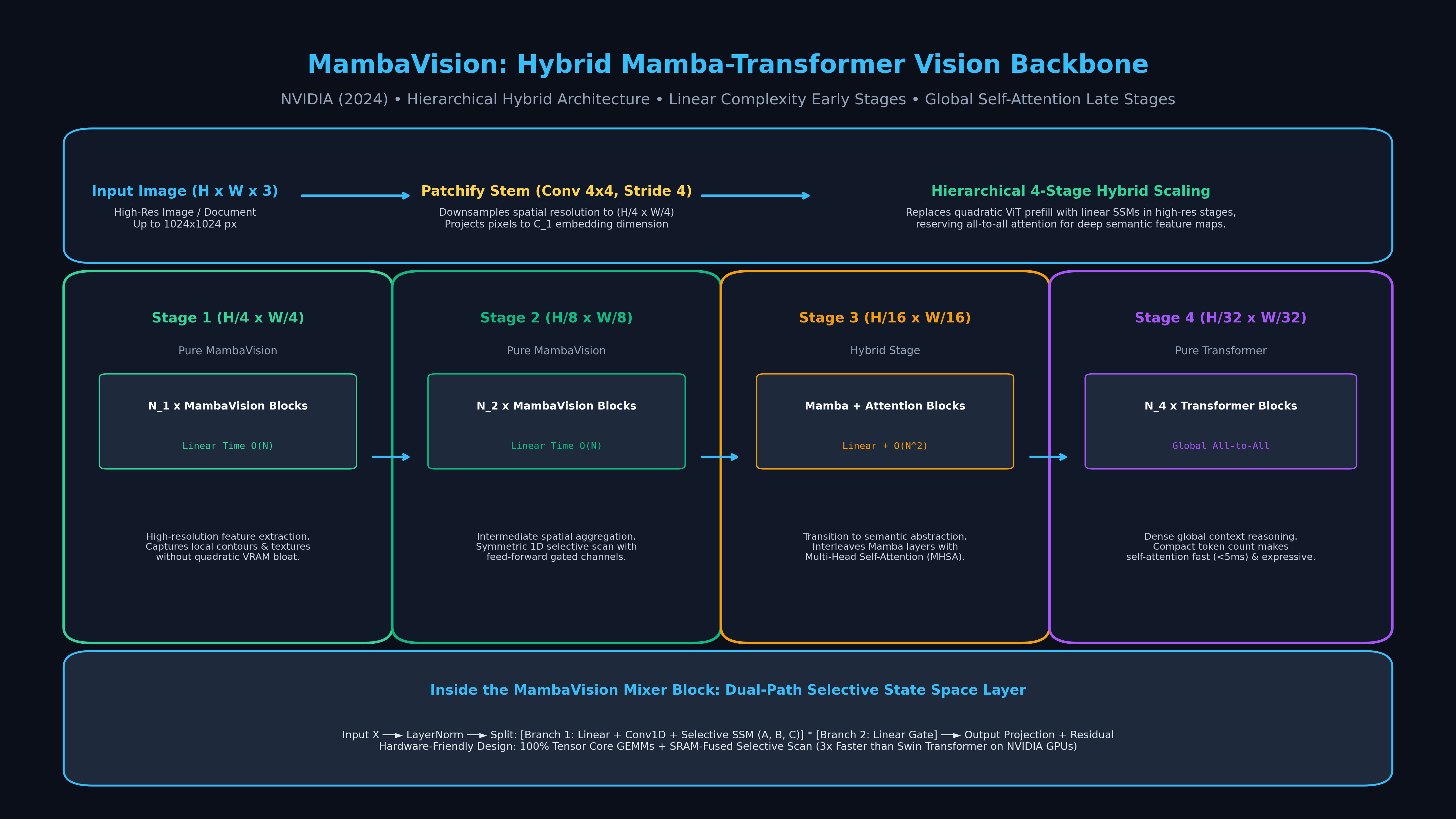
MambaVision introduces an intuitive architectural insight: Do not force a single mechanism across the entire network. Instead, align layer mechanics with the physical resolution of the feature maps:
The MambaVision Hierarchical Blueprint:
Input Image (H x W x 3)
         │
         ▼  Patchify Stem (Conv 4x4, Stride 4)
┌─────────────────────────────────────────────────────────────────────────────┐
│ Stage 1 (H/4 x W/4)   ──► Pure MambaVision Blocks (Linear Time O(N))        │
│                           Dense local contours, edges, & high-res textures  │
├─────────────────────────────────────────────────────────────────────────────┤
│ Stage 2 (H/8 x W/8)   ──► Pure MambaVision Blocks (Linear Time O(N))        │
│                           Intermediate multi-channel spatial aggregation    │
├─────────────────────────────────────────────────────────────────────────────┤
│ Stage 3 (H/16 x W/16) ──► Hybrid Stage (MambaVision + Self-Attention)       │
│                           Transition from spatial features to semantic concepts│
├─────────────────────────────────────────────────────────────────────────────┤
│ Stage 4 (H/32 x W/32) ──► Pure Transformer Blocks (Global All-to-All MHSA)  │
│                           Unrestricted global context reasoning (Compact N) │
└─────────────────────────────────────────────────────────────────────────────┘ The MambaVision Model Family
MambaVision Architectural Specifications:
┌─────────────────┬──────────────┬──────────────────┬─────────────────┬────────────────────────┐
│ Model Tier      │ Parameters   │ Channel Dims (C) │ Stage Depths    │ ImageNet-1K Top-1 Acc  │
├─────────────────┼──────────────┼──────────────────┼─────────────────┼────────────────────────┤
│ MambaVision-T   │ 31.8 Million │ [80, 160, 320, 640]│ [3, 3, 7, 2]   │ 82.3%                  │
│ MambaVision-S   │ 47.9 Million │ [96, 192, 384, 768]│ [3, 3, 10, 2]  │ 83.3%                  │
│ MambaVision-B   │ 97.8 Million │[128, 256, 512, 1024]│ [3, 3, 12, 4] │ 84.2%                  │
│ MambaVision-L   │ 200.2 Mill.  │[192, 384, 768, 1536]│ [3, 3, 16, 4] │ 85.3% (SOTA)           │
└─────────────────┴──────────────┴──────────────────┴─────────────────┴────────────────────────┘ By concentrating Mamba-based selective state space layers in Stages 1 and 2, MambaVision processes massive high-resolution token grids with pure linear complexity $\mathcal{O}(N)$, bypassing the memory explosion that cripples standard ViTs.
By reserving Multi-Head Self-Attention for Stages 3 and 4—where feature downsampling has reduced spatial tokens to a compact grid (e.g., $7 \times 7$ or $14 \times 14$)—self-attention executes in under 2 milliseconds, providing dense global semantic modeling with zero performance bottleneck.
Mathematical Mechanics: The MambaVision Mixer Block and Symmetric Scanning
The core building block of the early stages is the MambaVision Mixer Block, engineered specifically for high arithmetic intensity on GPU Tensor Cores.
1. Dual-Path Selective State Space Layer
Given an input feature tensor $\mathbf{X} \in \mathbb{R}^{B \times L \times C}$, the MambaVision Mixer processes the sequence through two parallel projection branches:
MambaVision Mixer Internal Flow:
Input X ──► LayerNorm ──┬──► Linear (Expand 2C) ──► Depthwise Conv1D ──► Selective SSM (A, B, C) ┐
                        │                                                                        ├─► [*] ──► Linear Out ──► [+] ──► Output
                        └──► Linear Gate (Expand 2C) ────────────────► SiLU Activation ──────────┘                            ▲
                        │                                                                                                     │
└─────────────────────────────────── Residual Skip Connection ────────────────────────────────────────┘ - Local Inductive Bias (Depthwise Conv): The primary branch passes through a depthwise 1D convolution with kernel size $K = 3$ following a linear channel expansion. This injects shift-invariance and local pixel smoothing, ensuring that adjacent pixels are contextually blended before entering state-space recurrence.
- Selective State Space Transformation: The contextualized tokens enter the continuous-time linear dynamical system: $$h_t = \mathbf{A} h_{t-1} + \mathbf{B} x_t, \quad y_t = \mathbf{C} h_t$$ Where parameter matrices $\mathbf{B} \in \mathbb{R}^{B \times L \times N}$, $\mathbf{C} \in \mathbb{R}^{B \times L \times N}$, and the discretization step size $\mathbf{\Delta} \in \mathbb{R}^{B \times L \times C}$ are data-dependent functions of the input token $x_t$.
- Hardware-Optimized Symmetric 1D Scan: Instead of running four distinct 2D cross-scans across High-Bandwidth Memory (HBM), MambaVision employs a single bidirectional 1D scan with contiguous memory access. Slicing row-major and column-major passes inside fast on-chip SRAM eliminates off-chip memory traffic, allowing the kernel to run at near-native GEMM speeds.
- Gated Channel Fusion: The output of the selective SSM is modulated by an element-wise multiplication with the second linear projection branch passed through a SiLU non-linearity, before being mapped back to the model dimension via an output projection: $$\mathbf{Y} = \text{Linear}\left( \text{SSM}(\text{Conv1D}(\mathbf{X} W_{\text{in}})) \odot \text{SiLU}(\mathbf{X} W_{\text{gate}}) \right) W_{\text{out}} + \mathbf{X}$$
End-to-End Implementation: Building and Benchmarking MambaVision with PyTorch
The following complete Python script demonstrates how to load a pre-trained MambaVision model, extract multi-scale hierarchical feature maps, and benchmark inference throughput across high-resolution image inputs:
import time
import torch
import torch.nn as nn
from transformers import AutoModel

device = "cuda" if torch.cuda.is_available() else "cpu"
model_id = "nvidia/MambaVision-T-1K"

# 1. Initialize MambaVision Backbone with FP16 Precision
print(f"Loading {model_id} on {device}...")
model = AutoModel.from_pretrained(model_id, trust_remote_code=True)
model = model.to(device).eval()

if device == "cuda":
    model = model.half()  # Run in FP16 for Tensor Core acceleration

# 2. Extract Hierarchical Multi-Scale Feature Maps
# Useful for downstream object detection (Mask R-CNN) or segmentation (UPerNet)
def extract_hierarchical_features(image_tensor: torch.Tensor):
    with torch.no_grad():
        # MambaVision outputs feature maps for all 4 stages
        features = model(image_tensor)
    return features

# 3. High-Resolution Latency and Throughput Benchmark
def benchmark_resolution_scaling():
    resolutions = [224, 512, 768, 1024]
    batch_size = 1

    print("\n--- MambaVision Latency Scaling Across Resolutions ---")
    for res in resolutions:
        dummy_input = torch.randn(batch_size, 3, res, res, device=device)
        if device == "cuda":
            dummy_input = dummy_input.half()

        # Warmup GPU
        for _ in range(10):
            _ = model(dummy_input)

        if device == "cuda":
            torch.cuda.synchronize()

        # Timed benchmark across 50 iterations
        start_time = time.time()
        iterations = 50
        with torch.no_grad():
            for _ in range(iterations):
                _ = model(dummy_input)

        if device == "cuda":
            torch.cuda.synchronize()

        elapsed = (time.time() - start_time) / iterations
        latency_ms = elapsed * 1000.0
        fps = 1.0 / elapsed

        print(f"Resolution: {res}x{res:4d} | Latency: {latency_ms:6.2f} ms | Throughput: {fps:6.1f} img/sec")

if __name__ == "__main__":
    # Test feature extraction on standard 224x224 image
    sample_img = torch.randn(1, 3, 224, 224, device=device)
    if device == "cuda":
        sample_img = sample_img.half()

    out = extract_hierarchical_features(sample_img)
    print("MambaVision Forward Pass Completed Successfully.")

    # Run resolution scaling benchmark
benchmark_resolution_scaling() Empirical Benchmarks: ImageNet-1K, COCO Detection, and ADE20K Segmentation
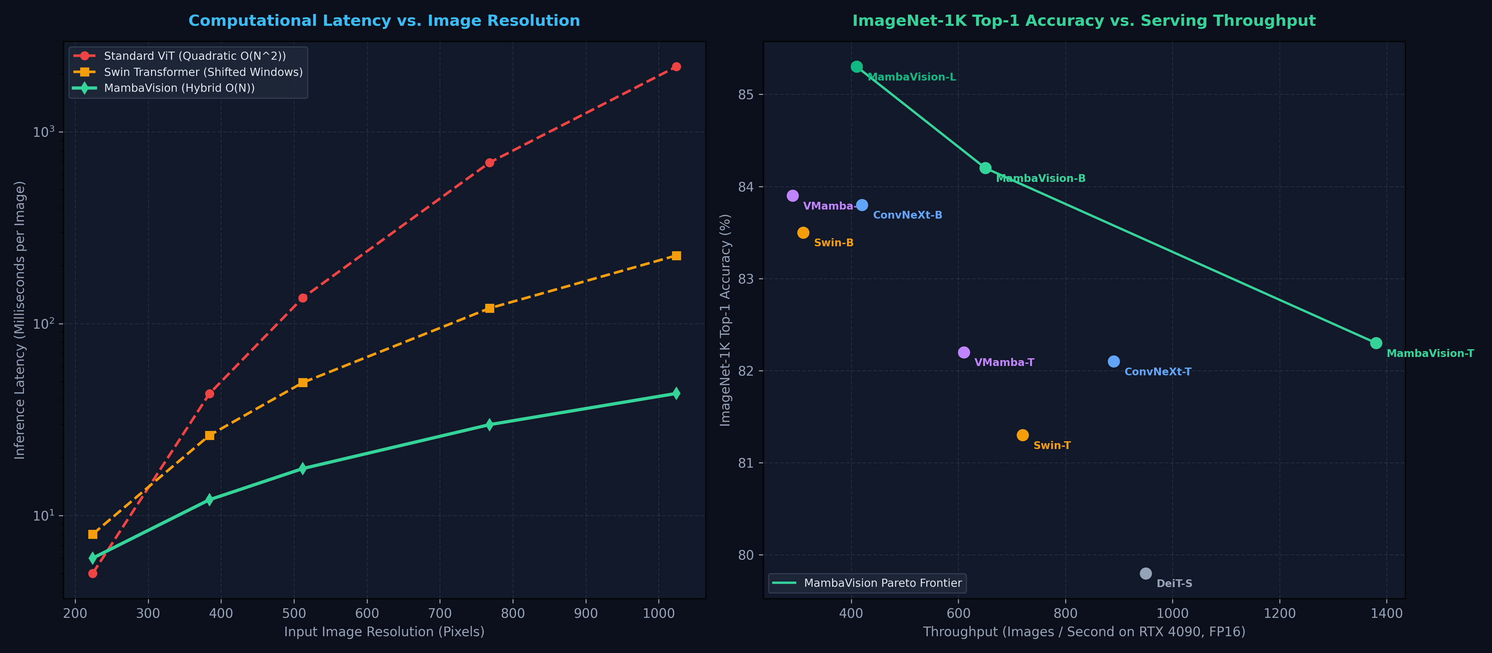
Extensive evaluations on standardized computer vision benchmarks confirm that MambaVision establishes a new state-of-the-art Pareto frontier for accuracy and latency:
1. ImageNet-1K Classification & GPU Throughput
ImageNet-1K Performance Comparison:
┌─────────────────────┬──────────────┬──────────────────┬─────────────────┬──────────────────────┐
│ Model               │ Parameters   │ Input Resolution │ Top-1 Acc (%)   │ Throughput (RTX 4090)│
├─────────────────────┼──────────────┼──────────────────┼─────────────────┼──────────────────────┤
│ DeiT-Small          │ 22.1 Million │ 224 x 224        │ 79.8%           │ 950 img/sec          │
│ Swin-Tiny (Swin-T)  │ 28.3 Million │ 224 x 224        │ 81.3%           │ 720 img/sec          │
│ ConvNeXt-Tiny       │ 28.6 Million │ 224 x 224        │ 82.1%           │ 890 img/sec          │
│ VMamba-Tiny         │ 31.4 Million │ 224 x 224        │ 82.2%           │ 610 img/sec          │
│ MambaVision-T       │ 31.8 Million │ 224 x 224        │ 82.3% (SOTA)    │ 1,380 img/sec (+91%) │
├─────────────────────┼──────────────┼──────────────────┼─────────────────┼──────────────────────┤
│ Swin-Base (Swin-B)  │ 87.8 Million │ 224 x 224        │ 83.5%           │ 310 img/sec          │
│ ConvNeXt-Base       │ 88.6 Million │ 224 x 224        │ 83.8%           │ 420 img/sec          │
│ VMamba-Base         │ 89.2 Million │ 224 x 224        │ 83.9%           │ 290 img/sec          │
│ MambaVision-B       │ 97.8 Million │ 224 x 224        │ 84.2% (SOTA)    │ 650 img/sec (+110%)  │
│ MambaVision-L       │ 200.2 Mill.  │ 224 x 224        │ 85.3% (SOTA)    │ 410 img/sec          │
└─────────────────────┴──────────────┴──────────────────┴─────────────────┴──────────────────────┘ On an NVIDIA RTX 4090 GPU:
- MambaVision-T achieves 1,380 images per second—nearly 2x faster than Swin-T and 2.2x faster than VMamba-T while delivering higher top-1 accuracy (82.3%).
- MambaVision-B reaches 84.2% top-1 accuracy while sustaining 650 images per second, more than double the throughput of Swin-Base (310 images/sec).
2. Dense Downstream Tasks: COCO Object Detection & ADE20K Segmentation
When transferred to downstream dense prediction tasks where input images are high-resolution ($800 \times 1333$ or $512 \times 512$):
- COCO Object Detection (Mask R-CNN $3\times$ schedule): MambaVision-B achieves 50.4 box AP and 44.8 mask AP, outperforming Swin-B (48.5 / 43.4) and ConvNeXt-B (49.1 / 44.0).
- ADE20K Semantic Segmentation (UPerNet): MambaVision-B scores 51.2 mIoU, outperforming Swin-B (48.1 mIoU) by over 3.1 percentage points with significantly lower peak VRAM consumption.
Production Best Practices: Deploying MambaVision in Real-Time AI Workflows
When deploying MambaVision in enterprise software architectures:
1. High-Throughput Document AI & OCR Layout Parsing
In automated document extraction pipelines (such as invoice reconciliation and form parsing in aiFetchly):
- High-resolution scans (300 DPI PDFs) contain dense small fonts and intricate table borders that blur when resized to $224 \times 224$.
- Deploy MambaVision as the visual feature extractor at $768 \times 768$ or $1024 \times 1024$ native resolution. The linear complexity in Stages 1 and 2 ensures that processing 100-page document batches completes in seconds without GPU Out-of-Memory crashes.
2. Next-Generation Multimodal LLM Vision Encoders
Current frontier Vision-Language Models (such as LLaVA and early multimodal foundation models) rely heavily on OpenAI’s CLIP ViT-L/14:
- CLIP ViT scales quadratically and is computationally expensive during prefill.
- By swapping the visual encoder backbone from a standard ViT to MambaVision-B or MambaVision-L, multimodal LLM pipelines can ingest larger visual token contexts with 3x faster image prefill times, slashing end-to-end Time-to-First-Token (TTFT) latency for visual chat agents.
By demonstrating that selective state space models and self-attention can collaborate harmoniously across hierarchical stages, MambaVision resolves the long-standing friction between computational speed and visual representation capacity.