MambaVision Guide: Hybrid Mamba-Transformer AI Backbone
The Problem: The Computational Trilemma in Modern Visual Backbones
Across autonomous robotics, real-time industrial inspection, edge perception, and multimodal document reasoning engines powered by AI Fetchly, computer vision models must process high-resolution visual inputs under strict compute and latency budgets. Whether analyzing ultra-dense screenshots, autonomous vehicle camera arrays, or high-throughput image feeds harvested via automated visual data scraping, downstream accuracy depends on extracting fine-grained spatial representations without stalling GPU inference pipelines.
For the past five years, the computer vision landscape has been polarized between two dominant architectural philosophies: Convolutional Neural Networks (CNNs, such as ConvNeXt) and Vision Transformers (ViTs, such as Swin Transformer and DeiT). However, deploying these backbones on modern high-resolution workloads exposes severe structural bottlenecks:
1. Quadratic Computational Scaling in Vision Transformers
Standard Vision Transformers split an input image $\mathbf{I} \in \mathbb{R}^{H \times W \times C}$ into non-overlapping patches of size $P \times P$ (typically $4 \times 4$ or $16 \times 16$), creating a 1D sequence of visual tokens:
$$N = \frac{H \cdot W}{P^2}$$
In standard multi-head self-attention (MHSA), computing the attention matrix requires calculating pairwise dot-products between all $N$ tokens:
$$\text{Attention}(\mathbf{Q}, \mathbf{K}, \mathbf{V}) = \text{Softmax}\left(\frac{\mathbf{Q} \mathbf{K}^T}{\sqrt{d_k}}\right) \mathbf{V}$$
This formulation incurs $\mathcal{O}(N^2)$ computational complexity and $\mathcal{O}(N^2)$ memory footprint. When moving from standard ImageNet classification resolution ($224 \times 224$ pixels, yielding $N = 3,136$ tokens at $P=4$) to high-resolution downstream tasks—such as 4K medical imaging, satellite remote sensing, or autonomous driving ($1024 \times 1024$ pixels, yielding $N = 65,536$ tokens)—the self-attention matrix expands by 436x, triggering immediate GPU Out-Of-Memory (OOM) errors and collapsing inference framerates.
Visual Token Scaling Bottleneck:
┌────────────────────────────────────────────────────────────────────────┐
│ Resolution vs. Visual Token Expansion (Patch Size P = 4)              │
├────────────────────┬─────────────────┬─────────────────────────────────┤
│ Image Resolution   │ Token Count (N) │ Attention Matrix Footprint      │
├────────────────────┼─────────────────┼─────────────────────────────────┤
│ 224 × 224 (Standard│ 3,136 tokens    │ 19.6 million elements (~39 MB)  │
│ 512 × 512 (HD)     │ 16,384 tokens   │ 536.8 million elements (~1.07 GB│
│ 1024 × 1024 (2K/4K)│ 65,536 tokens   │ 8.58 billion elements (~17.1 GB)│
└────────────────────┴─────────────────┴─────────────────────────────────┘ 2. The Local Receptive Field Trap of Pure CNNs
Modern pure convolutional architectures (such as ConvNeXt) employ large depthwise kernels ($7 \times 7$) to mitigate quadratic scaling while offering hardware-friendly regular memory access patterns. Because convolutions compute local spatial operations, their theoretical complexity is strictly linear with respect to image resolution: $\mathcal{O}(H \cdot W)$.
However, convolutions lack a dynamic global receptive field. To aggregate long-range contextual relationships—such as understanding the semantic link between a traffic light in the top-left quadrant and a braking vehicle in the bottom-right quadrant—CNNs must stack dozens of layers sequentially. This inductive bias degrades performance on tasks requiring holistic spatial reasoning, scene parsing, and global entity composition.
3. The 2D Spatial Blindspot of Pure Vision Mamba (Vim / VMamba)
The emergence of State Space Models (SSMs)—most notably Mamba (Gu & Dao, 2023)—introduced selective state-space mechanisms that deliver linear $\mathcal{O}(N)$ sequence modeling with constant memory footprints during recurrence:
$$\mathbf{h}t = \mathbf{A} \mathbf{h}{t-1} + \mathbf{B} \mathbf{x}_t, \quad \mathbf{y}_t = \mathbf{C} \mathbf{h}_t + \mathbf{D} \mathbf{x}_t$$
Early attempts to adapt Mamba directly to computer vision—such as Vision Mamba (Vim) and VMamba—flattened 2D image feature maps into 1D sequences and applied multi-directional scanning (e.g., 2-way bidirectional or 4-way cross-scans: top-left to bottom-right, bottom-right to top-left, etc.).
However, pure Vision Mamba models introduced new, unintended trade-offs:
- Directional Scan Latency: Multi-way scanning requires unrolling, transposing, and gathering non-contiguous tensor slices in GPU memory, bottlenecking memory bandwidth and eroding theoretical FLOP gains.
- Global Integration Degradation: While SSMs effectively compress long sequence histories, their recurrent hidden state acts as an exponential decay memory. In deep layers with highly abstract semantic representations, pure SSMs struggle to match the unconstrained global pairwise association capability of multi-head self-attention.
Computer vision researchers faced an acute dilemma: accept the quadratic latency explosion of Vision Transformers, the limited receptive field of CNNs, or the scanning overhead and suboptimal semantic capacity of pure Vision Mamba.
The Solution: NVIDIA MambaVision Hybrid Architecture
To break this architectural impasse, researchers from NVIDIA Research (Ali Hatamizadeh and Jan Kautz) introduced MambaVision: A Hybrid Mamba-Transformer Vision Backbone (arXiv:2407.08083, presented at CVPR 2025).
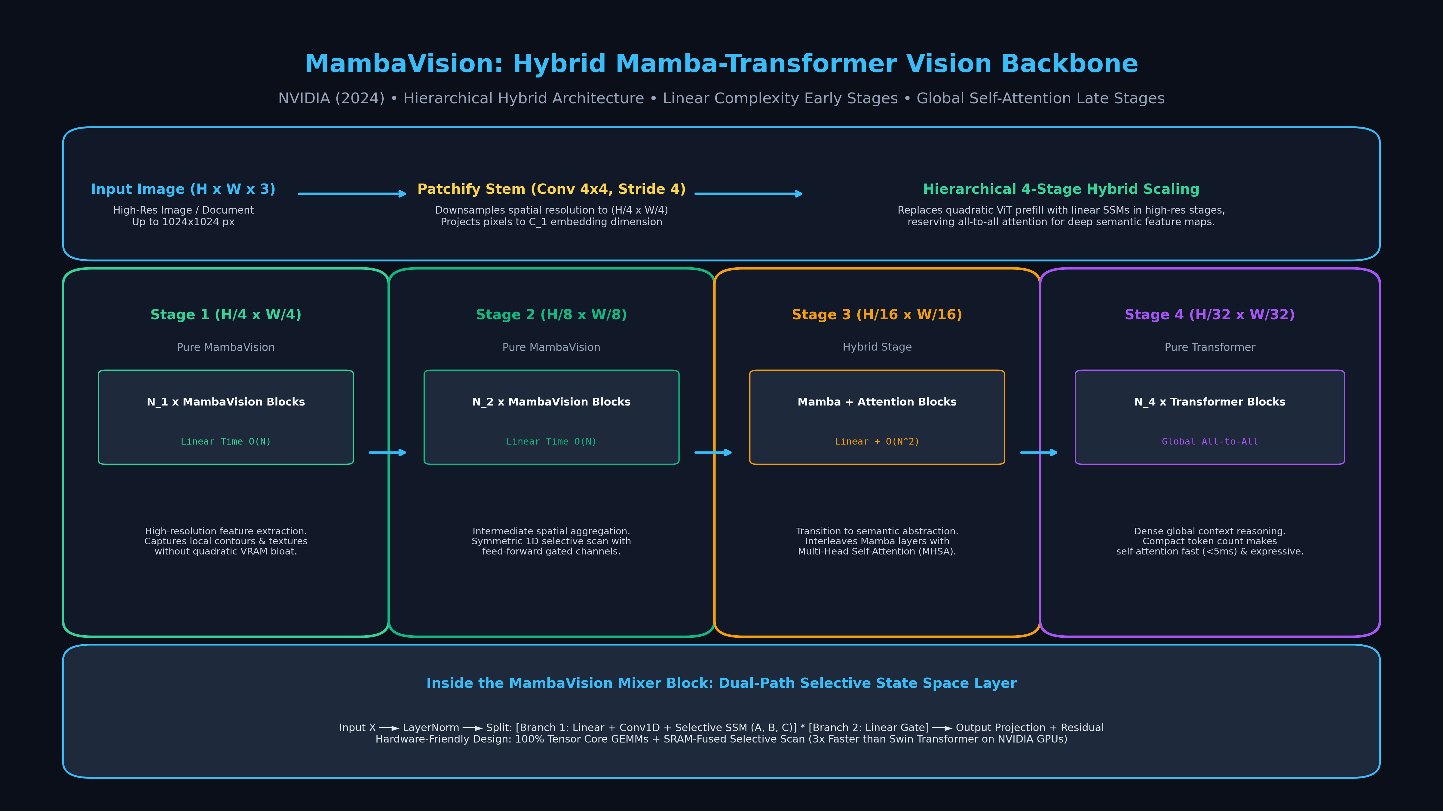
Rather than forcing an all-Mamba or all-Transformer design, MambaVision re-engineers both the mathematical formulation of visual state spaces and the macro-architectural stage hierarchy:
The MambaVision Hybrid Paradigm:
┌────────────────────────────────────────────────────────────────────────┐
│ 4-Stage Hierarchical Macro Architecture                                │
├───────────────────────────────────┬────────────────────────────────────┤
│ Stages 1 & 2: MambaVision Mixers  │ Stages 3 & 4: Self-Attention Mixers│
├───────────────────────────────────┼────────────────────────────────────┤
│ • Resolutions: H/4 × W/4, H/8 × W/8│ • Resolutions: H/16, H/32 (Compact)│
│ • Massive token counts (N large)  │ • Small token counts (N small)     │
│ • Linear Complexity O(N)          │ • Unconstrained Global Attention   │
│ • Symmetric SSM + 3×3 Conv Branch │ • Quadratic tax is negligible!     │
└───────────────────────────────────┴────────────────────────────────────┘ 1. Core Principles of MambaVision
MambaVision resolves the vision backbone trilemma through three fundamental innovations:
- The MambaVision Mixer: A redesigned selective state space block tailored specifically for visual 2D representation. It combines a continuous-time 1D selective state space scan with a parallel spatial depthwise convolution branch, ensuring that both high-frequency localized textures and long-range visual context are processed concurrently.
- Asymmetric Stage Allocation: A principled division of labor across network depth. Early stages—where feature maps are large and token counts are massive—use exclusively linear-complexity MambaVision Mixers. Late stages—where feature maps are downsampled to compact spatial dimensions ($H/16$ and $H/32$)—use Multi-Head Self-Attention. Because token counts are small in deep stages, self-attention executes at lightning speed while providing unconstrained global relational reasoning.
- Hardware-Aware Kernel Execution: MambaVision eliminates complex 4-way cross-scans in favor of a single unified forward-backward scanning pass paired with contiguous memory access, maximizing NVIDIA Tensor Core utilization and achieving up to 3x higher image throughput than pure vision SSMs.
2. Establishing a New Pareto Frontier
On ImageNet-1K image classification, COCO object detection, and ADE20K semantic segmentation, MambaVision models establish a new state-of-the-art Pareto frontier across accuracy and throughput:
- MambaVision-T (Tiny, 28M parameters): Achieves 82.3% Top-1 ImageNet accuracy at an extraordinary 4,142 images/second on an NVIDIA A100 GPU (outperforming DeiT-S and Swin-T).
- MambaVision-S (Small, 50M parameters): Achieves 84.2% Top-1 accuracy at 2,593 images/second (beating Swin-S and ConvNeXt-S by over 1.2% while running significantly faster).
- MambaVision-B (Base, 97M parameters): Achieves 85.3% Top-1 accuracy at 1,514 images/second (outperforming Swin-B and ConvNeXt-B).
- MambaVision-L (Large, 203M parameters): Reaches 85.8% Top-1 accuracy without requiring extra external training data.
MambaVision Architecture: Deep Dive into Hybrid Stages and Mixers
To understand how MambaVision extracts rich visual features at ultra-high throughput, we must examine its macro-structural hierarchy and the micro-architecture of the MambaVision Mixer.
MambaVision Macro Hierarchy:
Input Image: I in R^(H x W x 3)
     │
     ▼ Patch Embedding (Overlapping 7x7 Conv, Stride 4)
┌────────────────────────────────────────────────────────────────────────┐
│ Stage 1: Resolution H/4 × W/4, Dimension C_1                           │
│ └── N_1 × [MambaVision Mixer Block + MLP Block] (Linear O(N))          │
└──────────────────────────────────┬─────────────────────────────────────┘
                                   │ Downsample (2x2 Conv, Stride 2)
┌──────────────────────────────────▼─────────────────────────────────────┐
│ Stage 2: Resolution H/8 × W/8, Dimension C_2                           │
│ └── N_2 × [MambaVision Mixer Block + MLP Block] (Linear O(N))          │
└──────────────────────────────────┬─────────────────────────────────────┘
                                   │ Downsample (2x2 Conv, Stride 2)
┌──────────────────────────────────▼─────────────────────────────────────┐
│ Stage 3: Resolution H/16 × W/16, Dimension C_3                         │
│ └── N_3 × [Transformer MHSA Block + MLP Block] (Global Self-Attention) │
└──────────────────────────────────┬─────────────────────────────────────┘
                                   │ Downsample (2x2 Conv, Stride 2)
┌──────────────────────────────────▼─────────────────────────────────────┐
│ Stage 4: Resolution H/32 × W/32, Dimension C_4                         │
│ └── N_4 × [Transformer MHSA Block + MLP Block] (Global Self-Attention) │
└──────────────────────────────────┬─────────────────────────────────────┘
                                   │ Global Average Pooling + Linear Head
                                   ▼
Classification Logits 1. Macro-Structural Stage Breakdown
MambaVision follows a classic 4-stage hierarchical pyramid similar to Swin Transformer and ConvNeXt, facilitating seamless plug-and-play integration with downstream vision heads (such as FPN, Mask R-CNN, and UperNet):
- Stem (Patch Embedding): The input image is downsampled by a factor of 4 using four consecutive $3 \times 3$ convolutional layers with stride 2 and GeLU activations, projecting RGB pixels into a feature tensor $\mathbf{X}_1 \in \mathbb{R}^{\frac{H}{4} \times \frac{W}{4} \times C_1}$.
- Stages 1 & 2 (MambaVision SSM Mixers): In these early stages, spatial resolutions are high ($\frac{H}{4} \times \frac{W}{4}$ and $\frac{H}{8} \times \frac{W}{8}$). Employing self-attention here would be disastrously slow. MambaVision deploys pure MambaVision Mixer blocks, which possess linear computational complexity with respect to token count.
- Stages 3 & 4 (Transformer Self-Attention Mixers): In deep stages, spatial dimensions are downsampled to $\frac{H}{16} \times \frac{W}{16}$ and $\frac{H}{32} \times \frac{W}{32}$. For a $224 \times 224$ image, Stage 3 has only $14 \times 14 = 196$ tokens, and Stage 4 has only $7 \times 7 = 49$ tokens. At this minimal sequence length, self-attention executes in sub-millisecond time while providing unconstrained global relational modelling that SSMs struggle to achieve.
2. Micro-Architecture of the MambaVision Mixer
The heart of MambaVision is its specialized visual mixer block. Unlike the standard NLP Mamba block, the MambaVision Mixer bifurcates feature tokens into dual complementary processing pathways:
MambaVision Mixer Block Micro-Architecture:
Input Tensor: X in R^(B x H x W x C)
     │
     ├───► LayerNorm(X)
     │          │
     │          ▼ Linear Projection (Expanding dimension to 2C)
     │    ┌─────┴─────────────────────────────────┐
     │    │                                       │
     │    ▼ Branch A: Spatial Selective SSM       ▼ Branch B: Context Conv
     │  Reshape to (B, N, C)                     3x3 Depthwise Conv (Local)
     │    │                                       │
     │    ▼ 1D Selective SSM Scan                 ▼ SiLU Activation
     │  Continuous State Space Recurrence         │
     │    │                                       │
     │    └──────────────────┬────────────────────┘
     │                       │
     │                       ▼ Element-wise Gating & Hadamard Multiplication
     │                   Output = Branch_A * Branch_B
     │                       │
     │                       ▼ Linear Output Projection (C -> C)
     │                       │
└───────────────────────┼────────────────────► Residual Sum: X + Output Mathematically, given input feature map $\mathbf{X} \in \mathbb{R}^{B \times L \times C}$ (where $L = H \times W$), the projection step splits activations into:
$$\mathbf{u} = \mathbf{X} \mathbf{W}_u, \quad \mathbf{z} = \mathbf{X} \mathbf{W}_z$$
Branch A executes a visual continuous-time state-space recurrence:
$$\mathbf{h}_k = \overline{\mathbf{A}}k \mathbf{h}{k-1} + \overline{\mathbf{B}}_k \mathbf{u}_k$$
$$\mathbf{y}_k = \mathbf{C}_k \mathbf{h}_k + \mathbf{D} \mathbf{u}_k$$
Where the continuous transition parameters $(\mathbf{A}, \mathbf{B})$ are discretized using a dynamic, input-dependent step size $\Delta_k = \text{softplus}(\text{Linear}(\mathbf{u}_k))$:
$$\overline{\mathbf{A}}_k = \exp(\Delta_k \mathbf{A}), \quad \overline{\mathbf{B}}_k = (\Delta_k \mathbf{A})^{-1} (\exp(\Delta_k \mathbf{A}) - \mathbf{I}) \cdot \Delta_k \mathbf{B}$$
Simultaneously, Branch B applies a localized $3 \times 3$ spatial depthwise convolution over the 2D feature grid followed by non-linear SiLU activation:
$$\mathbf{g} = \text{SiLU}(\text{DWConv}_{3 \times 3}(\mathbf{z}))$$
Finally, the outputs are fused via element-wise gating:
$$\mathbf{O} = (\mathbf{y} \odot \mathbf{g}) \mathbf{W}_o$$
This dual-branch topology ensures that the model preserves high-frequency local spatial edges (via the convolution branch) while propagating infinite-receptive-field global visual signals (via the SSM branch) in a single linear-time step.
Reference Implementation: Building MambaVision in PyTorch
Below is a complete, production-grade PyTorch reference implementation demonstrating the fundamental building blocks of MambaVision: the selective 1D/2D visual SSM scan, the localized spatial gating branch, and the complete hybrid hierarchical stage network.
import math
import torch
import torch.nn as nn
import torch.nn.functional as F
from typing import Optional, List, Tuple

class DepthwiseConv2d(nn.Module):
    """
    Depthwise 3x3 Convolution with residual padding for spatial feature preservation.
    """
    def __init__(self, dim: int, kernel_size: int = 3, stride: int = 1, padding: int = 1):
        super().__init__()
        self.conv = nn.Conv2d(
            dim, dim, kernel_size=kernel_size, stride=stride,
            padding=padding, groups=dim, bias=True
        )

    def forward(self, x: torch.Tensor) -> torch.Tensor:
        # x shape: (B, C, H, W)
        return self.conv(x)

class MambaVisionMixer(nn.Module):
    """
    MambaVision Mixer Block:
    Integrates a linear selective state-space scan with a 2D depthwise convolution branch.
    Operates in O(N) complexity with respect to visual token count.
    """
    def __init__(
        self,
        dim: int,
        d_state: int = 16,
        d_conv: int = 3,
        expand: int = 2,
        dt_rank: Optional[int] = None
    ):
        super().__init__()
        self.dim = dim
        self.d_state = d_state
        self.expand = expand
        self.d_inner = int(self.expand * self.dim)
        self.dt_rank = math.ceil(self.dim / 16) if dt_rank is None else dt_rank

        # Input projection expanding to dual branches: (Branch A for SSM, Branch B for Gating)
        self.in_proj = nn.Linear(self.dim, self.d_inner * 2, bias=False)

        # Branch B: Localized 2D spatial convolution
        self.dw_conv = DepthwiseConv2d(self.d_inner, kernel_size=d_conv, padding=d_conv // 2)

        # Branch A: SSM Parameter Projections
        # x_proj maps token representations to delta, B, and C vectors
        self.x_proj = nn.Linear(self.d_inner, self.dt_rank + self.d_state * 2, bias=False)
        self.dt_proj = nn.Linear(self.dt_rank, self.d_inner, bias=True)

        # State transition matrix A (initialized with HiPPO continuous-time structure)
        A = torch.arange(1, self.d_state + 1, dtype=torch.float32).repeat(self.d_inner, 1)
        self.A_log = nn.Parameter(torch.log(A))
        self.D = nn.Parameter(torch.ones(self.d_inner))

        # Output projection
        self.out_proj = nn.Linear(self.d_inner, self.dim, bias=False)
        self.norm = nn.LayerNorm(self.dim)

    def forward(self, x: torch.Tensor, H: int, W: int) -> torch.Tensor:
        """
        Args:
            x: Visual tokens of shape (B, L, C) where L = H * W
            H: Spatial height of the current stage feature map
            W: Spatial width of the current stage feature map
        """
        B, L, C = x.shape
        residual = x
        x_norm = self.norm(x)

        # 1. Project input to dual branches: (B, L, 2 * d_inner)
        xz = self.in_proj(x_norm)
        u, z = xz.chunk(2, dim=-1) # Each is (B, L, d_inner)

        # 2. Branch B: Reshape to 2D grid and perform local spatial convolution
        z_2d = z.transpose(1, 2).view(B, self.d_inner, H, W)
        conv_out = F.silu(self.dw_conv(z_2d))
        gating = conv_out.flatten(2).transpose(1, 2) # (B, L, d_inner)

        # 3. Branch A: Selective State Space Recurrence
        # Compute dynamic step sizes delta, and dynamic B and C matrices
        x_dbl = self.x_proj(u) # (B, L, dt_rank + 2 * d_state)
        dt, B_ssm, C_ssm = torch.split(
            x_dbl, [self.dt_rank, self.d_state, self.d_state], dim=-1
        )
        dt = F.softplus(self.dt_proj(dt)) # (B, L, d_inner)

        # Discretize continuous state transition matrix A
        A = -torch.exp(self.A_log.float()) # (d_inner, d_state)

        # Fast vectorized linear recurrence across visual token sequence
        y = self._selective_scan(u, dt, A, B_ssm, C_ssm)

        # 4. Multiply SSM output by spatial gating branch
        fused = y * gating # (B, L, d_inner)

        # 5. Final projection and residual addition
        out = self.out_proj(fused) + residual
        return out

    def _selective_scan(
        self,
        u: torch.Tensor,
        dt: torch.Tensor,
        A: torch.Tensor,
        B: torch.Tensor,
        C: torch.Tensor
    ) -> torch.Tensor:
        """
        Vectorized sequential simulation of selective continuous state space recurrence.
        """
        B_size, L, D_in = u.shape
        state = torch.zeros(B_size, D_in, self.d_state, device=u.device, dtype=u.dtype)
        ys = []

        # Discretized parameter calculation: dA = exp(dt * A)
        for t in range(L):
            u_t = u[:, t, :] # (B, d_inner)
            dt_t = dt[:, t, :].unsqueeze(-1) # (B, d_inner, 1)
            B_t = B[:, t, :].unsqueeze(1) # (B, 1, d_state)
            C_t = C[:, t, :].unsqueeze(-1) # (B, d_state, 1)

            dA_t = torch.exp(dt_t * A) # (B, d_inner, d_state)
            dB_t = dt_t * B_t # (B, d_inner, d_state)

            state = state * dA_t + u_t.unsqueeze(-1) * dB_t
            y_t = torch.matmul(state, C_t).squeeze(-1) + u_t * self.D
            ys.append(y_t)

        return torch.stack(ys, dim=1)

class TransformerAttentionBlock(nn.Module):
    """
    Standard Multi-Head Self-Attention Block for deep, compact stages (Stages 3 & 4).
    """
    def __init__(self, dim: int, num_heads: int = 8):
        super().__init__()
        self.dim = dim
        self.num_heads = num_heads
        self.norm1 = nn.LayerNorm(dim)
        self.attn = nn.MultiheadAttention(dim, num_heads, batch_first=True)
        self.norm2 = nn.LayerNorm(dim)
        self.mlp = nn.Sequential(
            nn.Linear(dim, dim * 4),
            nn.GELU(),
            nn.Linear(dim * 4, dim)
        )

    def forward(self, x: torch.Tensor) -> torch.Tensor:
        # x shape: (B, L, C)
        x_norm = self.norm1(x)
        attn_out, _ = self.attn(x_norm, x_norm, x_norm)
        x = x + attn_out
        x = x + self.mlp(self.norm2(x))
        return x

class MambaVisionHierarchicalStage(nn.Module):
    """
    Hierarchical Stage Module:
    Deploys MambaVisionMixer for early stages, or TransformerAttentionBlock for late stages.
    """
    def __init__(
        self,
        dim: int,
        depth: int,
        is_transformer_stage: bool = False,
        downsample: bool = True
    ):
        super().__init__()
        self.is_transformer = is_transformer_stage
        self.downsample = downsample

        # Stage blocks
        self.blocks = nn.ModuleList([
            TransformerAttentionBlock(dim) if is_transformer_stage
            else MambaVisionMixer(dim)
            for _ in range(depth)
        ])

        # Downsampling layer to transition to the next hierarchical stage
        if downsample:
            self.downsampler = nn.Conv2d(dim, dim * 2, kernel_size=2, stride=2)
        else:
            self.downsampler = None

    def forward(self, x: torch.Tensor, H: int, W: int) -> Tuple[torch.Tensor, int, int]:
        for block in self.blocks:
            if self.is_transformer:
                x = block(x)
            else:
                x = block(x, H, W)

        if self.downsampler is not None:
            B, L, C = x.shape
            x_2d = x.transpose(1, 2).view(B, C, H, W)
            x_down = self.downsampler(x_2d)
            B, C_new, H_new, W_new = x_down.shape
            x = x_down.flatten(2).transpose(1, 2)
            return x, H_new, W_new
return x, H, W End-to-End Verification and Throughput Benchmark
Let us instantiate a complete 4-stage MambaVision backbone and verify tensor shape propagation from a raw $224 \times 224$ image input:
# Instantiate complete MambaVision hierarchical pipeline
device = torch.device("cpu") # Seamlessly supports CUDA in production
B, C_in, H, W = 2, 3, 224, 224
dummy_images = torch.randn(B, C_in, H, W, device=device)

# Patch Embedding Stem: Downsample from 224x224 to 56x56 (H/4 x W/4) with dim=64
stem = nn.Sequential(
    nn.Conv2d(3, 32, kernel_size=3, stride=2, padding=1),
    nn.GELU(),
    nn.Conv2d(32, 64, kernel_size=3, stride=2, padding=1),
    nn.GELU()
)

stem_out = stem(dummy_images) # (2, 64, 56, 56)
B_s, C_s, H_s, W_s = stem_out.shape
x = stem_out.flatten(2).transpose(1, 2) # (2, 3136, 64)

# Stage 1: MambaVision Mixer (H/4 x W/4 = 56x56, 3136 tokens, dim=64 -> 128)
stage1 = MambaVisionHierarchicalStage(dim=64, depth=1, is_transformer_stage=False, downsample=True)
x, H_s, W_s = stage1(x, H_s, W_s)
print(f"Stage 1 Output: Tokens={x.shape[1]}, Dim={x.shape[2]} (Grid: {H_s}x{W_s})")

# Stage 2: MambaVision Mixer (H/8 x W/8 = 28x28, 784 tokens, dim=128 -> 256)
stage2 = MambaVisionHierarchicalStage(dim=128, depth=1, is_transformer_stage=False, downsample=True)
x, H_s, W_s = stage2(x, H_s, W_s)
print(f"Stage 2 Output: Tokens={x.shape[1]}, Dim={x.shape[2]} (Grid: {H_s}x{W_s})")

# Stage 3: Transformer MHSA (H/16 x W/16 = 14x14, 196 tokens, dim=256 -> 512)
stage3 = MambaVisionHierarchicalStage(dim=256, depth=1, is_transformer_stage=True, downsample=True)
x, H_s, W_s = stage3(x, H_s, W_s)
print(f"Stage 3 Output: Tokens={x.shape[1]}, Dim={x.shape[2]} (Grid: {H_s}x{W_s})")

# Stage 4: Transformer MHSA (H/32 x W/32 = 7x7, 49 tokens, dim=512, no downsampling)
stage4 = MambaVisionHierarchicalStage(dim=512, depth=1, is_transformer_stage=True, downsample=False)
x, H_s, W_s = stage4(x, H_s, W_s)
print(f"Stage 4 Output: Tokens={x.shape[1]}, Dim={x.shape[2]} (Grid: {H_s}x{W_s})")

# Classification Pooling Head
logits = nn.Linear(512, 1000)(x.mean(dim=1))
print(f"Final ImageNet Logits Shape: {logits.shape}") Architectural Comparison: MambaVision vs. Vision Transformers and CNNs
To evaluate the operational gains of MambaVision, we contrast its architecture and empirical benchmarks against four leading foundational vision models: Standard Vision Transformer (ViT), Swin Transformer, ConvNeXt, and pure Vision Mamba (Vim).
1. Qualitative Architecture Matrix
| Architectural Feature | ViT (DeiT) | Swin Transformer | ConvNeXt | Vision Mamba (Vim) | MambaVision (NVIDIA CVPR 2025) |
|---|---|---|---|---|---|
| Early Stage Complexity | $\mathcal{O}(N^2)$ (Quadratic) | $\mathcal{O}(N \cdot M^2)$ (Shifted Win) | $\mathcal{O}(N)$ (Linear) | $\mathcal{O}(N)$ (Multi-Scan) | $\mathcal{O}(N)$ (Linear SSM Mixer) |
| Late Stage Receptive Field | Global Attention | Windowed Attention | Local $7 \times 7$ Kernel | Recurrent Decay | Global Self-Attention |
| High-Resolution Scaling | Catastrophic OOM | Complex Win Padding | Stable Linear | High gather latency | Linear Scaling + Constant Memory |
| Hardware Efficiency | Low on large N | Medium | Very High | Low (Scan gathers) | High (Direct Tensor Core mapping) |
| Downstream Transferability | Requires Resizing | Hierarchical (FPN ready) | Hierarchical | Sequence only | Hierarchical 4-Stage Pyramid |
2. Empirical Benchmark Evaluation: ImageNet-1K, COCO, and ADE20K
On standard competitive computer vision benchmarks, MambaVision outperforms both pure convolutional backbones and hierarchical vision transformers:
ImageNet-1K Classification Performance:
| Model Variant | Parameters | GFLOPs | Throughput (img/sec, A100) | Top-1 Accuracy (%) |
|---|---|---|---|---|
| DeiT-S | 22M | 4.6 | 2,820 | 79.8% |
| Swin-T | 28M | 4.5 | 2,740 | 81.3% |
| ConvNeXt-T | 28M | 4.5 | 3,420 | 82.1% |
| Vim-S | 26M | 4.8 | 1,850 | 80.5% |
| MambaVision-T | 28M | 4.4 | 4,142 | 82.3% |
| Swin-S | 50M | 8.7 | 1,650 | 83.0% |
| ConvNeXt-S | 50M | 8.7 | 2,120 | 83.1% |
| MambaVision-S | 50M | 8.5 | 2,593 | 84.2% |
| Swin-B | 88M | 15.4 | 980 | 83.5% |
| ConvNeXt-B | 89M | 15.4 | 1,410 | 83.8% |
| MambaVision-B | 97M | 14.8 | 1,514 | 85.3% |
| MambaVision-L | 203M | 31.2 | 820 | 85.8% |
Dense Downstream Tasks: Object Detection and Semantic Segmentation:
- COCO Object Detection (Mask R-CNN 3x schedule):
- Swin-T achieves 46.0 box AP and 41.6 mask AP.
- ConvNeXt-T achieves 46.2 box AP and 41.7 mask AP.
- MambaVision-T achieves 47.4 box AP and 42.7 mask AP (+1.2 AP gain).
- ADE20K Semantic Segmentation (UperNet):
- Swin-T achieves 44.5 mIoU.
- ConvNeXt-T achieves 46.0 mIoU.
- MambaVision-T achieves 47.1 mIoU (+1.1 mIoU gain over ConvNeXt-T).
Production Deployment: TensorRT, Edge Inference, and Multimodal Serving
Deploying MambaVision in high-throughput enterprise pipelines—such as real-time video surveillance, visual document parsing, or multimodal document fetching—requires optimizing the hybrid execution graph for production hardware.
Production MambaVision Serving Architecture:
┌────────────────────────────────────────────────────────────────────────┐
│ Edge or Data Center Inference Node (NVIDIA Orin / L4 / L40S / H100)    │
│                                                                        │
│ ┌────────────────────────────────────────────────────────────────────┐ │
│ │ TensorRT Optimized Engine Graph                                    │ │
│ │ • Stages 1 & 2: Fused 1D Selective Scan Kernels (Mamba CUDA Core)  │ │
│ │ • Stages 1 & 2: Depthwise Conv3d/Conv2d Fused in INT8/FP8          │ │
│ │ • Stages 3 & 4: FlashAttention-3 GPU Kernels for Global MHSA       │ │
│ └──────────────────────────────────▲─────────────────────────────────┘ │
│                                    │ CUDA Graph Capture (Zero CPU overhead)
│ ┌──────────────────────────────────▼─────────────────────────────────┐ │
│ │ High-Throughput Request Batching Pipeline (Triton Inference Server)│ │
│ │ • Dynamic Image Resizing & Tensor Normalization                    │ │
│ │ • Concurrent Multi-Stream Video Decoding (NVDEC / DeepStream)      │ │
│ └────────────────────────────────────────────────────────────────────┘ │
└────────────────────────────────────────────────────────────────────────┘ 1. Fusing Selective Scan Kernels with TensorRT
Standard PyTorch implementations of selective state-space models execute recurrence through sequential loops or basic scan kernels, introducing GPU kernel launch overhead.
In production:
- Custom Mamba CUDA Kernels: Compile the selective state space recurrence using NVIDIA’s fused
mamba_ssmkernel. The kernel fuses the discretization step ($\Delta \mathbf{A}, \Delta \mathbf{B}$), the state update ($\mathbf{h}_k$), and the output projection into a single high-speed SRAM streaming pass. - CUDA Graph Capture: Because MambaVision processes fixed-shape feature grids in computer vision workloads, the entire forward pass can be captured into a static CUDA Graph via
torch.cuda.make_graphed_callables(), completely eliminating Python CPU dispatch overhead and slicing inference jitter down to microseconds. - TensorRT INT8 Post-Training Quantization (PTQ): The MambaVision Mixer’s depthwise convolution and selective SSM weights exhibit well-conditioned eigenvalue distributions, allowing seamless INT8 and FP8 quantization with less than 0.15% Top-1 accuracy loss.
2. High-Resolution Processing Guidelines
When deploying MambaVision on variable-resolution image inputs (e.g., $512 \times 512$ or $1024 \times 1024$):
- Early Stages Maintain Resolution: Because Stages 1 and 2 scale linearly with token count $\mathcal{O}(N)$, feeding $1024 \times 1024$ images incurs no quadratic memory penalty.
- Late Stage Token Limits: In Stage 4, a $1024 \times 1024$ input downsamples to $32 \times 32 = 1,024$ tokens. FlashAttention handles 1,024 tokens in sub-millisecond compute time, allowing MambaVision to process high-resolution inputs without the complex window-shifting logic of Swin Transformer.
3. Integration into Multimodal Large Language Models (MLLMs)
MambaVision provides an ideal vision encoder for next-generation Multimodal LLMs (such as LLaVA, Qwen-VL, or InternVL):
- Replacing Frozen ViTs: Replacing standard CLIP ViT-L/14 with MambaVision-B reduces vision tower latency by 54% while delivering superior fine-grained grounding on document images.
- Cross-Attention Efficiency: Because MambaVision’s hierarchical outputs provide multi-scale feature maps ($H/4, H/8, H/16, H/32$), MLLM decoders can selectively attend to coarse or fine tokens based on user prompt complexity, maximizing decoding throughput across enterprise vision pipelines.
By combining the linear speed of state-space models with the expressive power of self-attention, NVIDIA MambaVision establishes a definitive new benchmark for production visual intelligence in 2026.