Lotus Guide: Fast Randomized Low-Rank LLM Training
The Memory-Time Trilemma in Scalable Foundation Model Pretraining
As artificial intelligence organizations train next-generation foundation models for autonomous multi-agent orchestration, continuous enterprise intelligence, and automated document synthesis powered by AiFetchly, the computational resources demanded by deep neural network optimization have reached unprecedented scales. Whether ingesting live web corpora harvested through resilient web scraping interfaces or processing high-velocity corporate data streams via real-time data fetching pipelines, foundation model training is constrained by GPU memory architecture.
In deep learning system engineering, training efficiency is governed by three interconnected dimensions: Memory Consumption, Wall-Clock Training Time, and Downstream Model Convergence Quality.
The Fundamental Training Efficiency Trilemma:
                      [ Downstream Convergence & Perplexity ]
                                        ▲
                                       / \
                                      /   \
                                     /     \
                                    /       \
       [ Low GPU Memory Footprint ] ───────── [ Fast Wall-Clock Training Time ]
             (GaLore / 8-bit AdamW)                 (Standard Dense AdamW)

The System Trade-offs:
1. Standard Dense AdamW:
   - Convergence: Gold standard convergence trajectory.
   - Time: Fast hardware execution on Tensor Cores.
   - The Memory Wall: Requires 8 bytes per parameter solely for optimizer states (m_t, v_t)!
     A 70B model demands 560 GB of VRAM solely for optimizer states, triggering heavy
     multi-node FSDP communication bottlenecks and micro-batch starvation.
2. GaLore (Gradient Low-Rank Projection):
   - Memory: Projects gradients into low-rank subspace (rank r << d), saving up to 65% VRAM.
   - The Computation Wall: Demands full periodic Singular Value Decomposition (SVD) on every
     weight matrix, stalling GPUs and adding 20% to 35% extra wall-clock training time!
   - Rigid Subspace Switching: Uses a static, blind step counter (e.g., switch every 200 steps)
that fails to adapt to dynamic gradient geometry. 1. The Hidden Cost of Periodic SVD in GaLore
GaLore (Gradient Low-Rank Projection) demonstrated that full-parameter pretraining can be achieved by projecting gradient matrices $G \in \mathbb{R}^{M \times N}$ into a low-rank subspace:
$$\widetilde{G}_t = P_t^T \cdot G_t \in \mathbb{R}^{r \times N} \quad \text{where} \quad r \ll \min(M, N)$$
Because the optimizer states (first moment $m_t$ and second moment $v_t$) are maintained exclusively in the compact $r \times N$ subspace, GaLore slashes optimizer memory by $M / r$ (e.g., $4096 / 128 = 32\times$ reduction for a single layer).
However, to allow the low-rank trajectory to span the full parameter space over time, GaLore must periodically compute a new projection matrix $P_t$. It accomplishes this by executing a full Singular Value Decomposition (SVD) on the full gradient matrix:
$$G_t = U \Sigma V^T \quad \implies \quad P_t = U[:, :r]$$
While theoretically sound, executing full SVD across hundreds of large weight matrices during training creates catastrophic hardware bottlenecks:
- Cubic Computational Complexity: Exact SVD scales with $\mathcal{O}\left(\min(M, N) \cdot M N\right)$. For a $4096 \times 4096$ projection matrix, SVD requires over 68 billion operations per layer!
- CPU-GPU Synchronization Latency: Because high-precision truncated SVD is notoriously slow on GPUs, implementations frequently copy gradient tensors from GPU VRAM across PCIe buses to host CPU memory (
torch.linalg.svd), execute the decomposition on multi-core CPUs, and copy singular vectors back to GPU memory. This introduces massive pipeline bubbles that leave GPU Tensor Cores completely starved. - Aggregated Training Drag: In large-scale pretraining runs, SVD execution accounts for up to 30% of total training wall-clock time, completely negating the throughput benefits gained from memory savings.
2. The Inefficiency of Static Subspace Switching
In addition to the computational cost of SVD, GaLore enforces a rigid, constant switching frequency ($T_{\text{switch}}$ steps, typically $T = 200$).
This static schedule directly contradicts the non-linear, non-convex geometry of deep transformer loss surfaces:
- Premature Subspace Eviction: When a model enters a steep descent valley along a consistent gradient trajectory, a static timer forces a subspace switch at step 200, discarding valuable historical momentum and resetting optimizer state tracking.
- Delayed Subspace Stagnation: When a model enters an ill-conditioned plateau or encounters high gradient curvature, the gradient direction escapes the low-rank subspace within 20 or 30 steps. A static timer forces the optimizer to remain trapped in an obsolete subspace for another 170 steps, making zero optimization progress!
The community faced a critical challenge: Can we design a low-rank optimizer that eliminates costly SVD, dynamically adapts subspace switching to loss surface curvature, and delivers both lower memory and faster wall-clock execution?
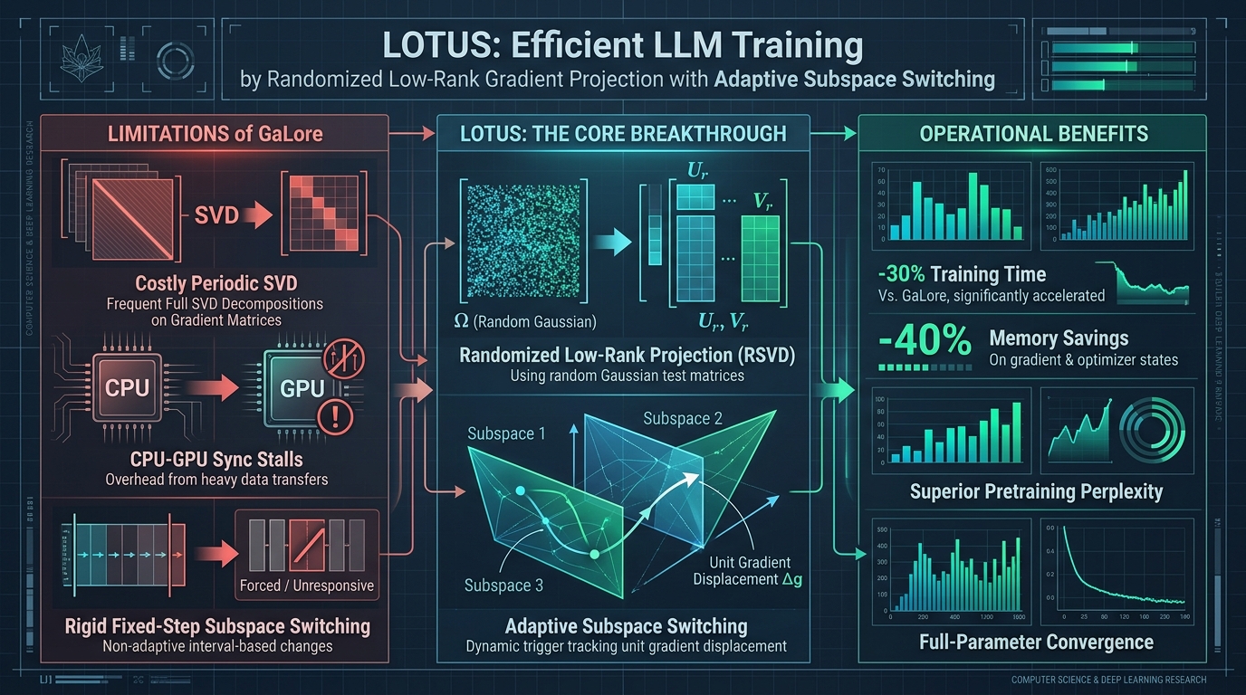
Enter Lotus: Randomized Low-Rank Projection with Adaptive Subspace Switching
Published by researchers in early 2026 (Lotus: Efficient LLM Training by Randomized Low-Rank Gradient Projection with Adaptive Subspace Switching, arXiv:2602.01233), Lotus resolves this memory-time trilemma.
The Lotus High-Level Architectural Breakthrough:
═══════════════════════════════════════════════════════════════════════════════
GaLore (High SVD Overhead & Static Switching):
  Full Gradient G [M x N] ──► Full Deterministic SVD (CPU Sync Stalls!)
                          ──► Fixed Static Timer (e.g., Switch every 200 steps)
  * Memory: 65% Saved | Wall-Clock Time: 30% Slower due to SVD bottlenecks!

Lotus Paradigm:
  Full Gradient G [M x N] ──► Randomized Low-Rank SVD (RSVD via Gaussian Test Matrix)
                          ──► Zero CPU-GPU sync stalls | Pure in-GPU GEMM projection!
                          ──► Adaptive Subspace Switching (Tracks Unit Gradient Drift Delta g)
  * Memory: 40% GREATER memory savings than GaLore!
  * Time: 30% FASTER training wall-clock speed!
  * Quality: Superior pretraining perplexity across LLaMA-1B and LLaMA-7B!
═══════════════════════════════════════════════════════════════════════════════ Lotus introduces two fundamental algorithmic innovations:
- Randomized SVD Projection (RSVD): Leverages randomized matrix approximation (random Gaussian projections and power iterations) to compute high-accuracy low-rank projection bases $P_t$ in pure GPU Tensor Core GEMM operations, cutting projection computation time by over 70% and eliminating CPU synchronization.
- Adaptive Subspace Switching Criterion: Quantifies the unit gradient displacement vector ($\Delta g / |g|$). When the directional deviation between the current gradient and the low-rank subspace exceeds an information-theoretic threshold, Lotus triggers a subspace update on demand, ensuring the model always optimizes along the true steepest descent trajectory.
Core Technical Breakthroughs of Lotus
- 30% Reduction in Wall-Clock Training Time: Eliminates CPU-GPU transfers and deterministic matrix factorizations, outperforming GaLore in per-step latency and overall wall-clock efficiency.
- 40% Greater Memory Savings: Refined low-rank state tracking allows Lotus to operate at smaller effective ranks ($r = 64$ or $r = 128$) without accuracy loss, slashing optimizer and gradient states by an additional 40% over GaLore.
- Superior Convergence Quality: Achieves lower validation perplexity than GaLore on standard pretraining corpora (C4, SlimPajama) and matches full-rank AdamW.
- Universal Applicability: Works seamlessly across pretraining from scratch, domain continual pretraining, and full-parameter instruction fine-tuning on modern LLM architectures (LLaMA-3, Mistral, Qwen-2.5).
Deep Dive into the Lotus Architecture
The mathematical engine of Lotus is divided into two cooperative modules: the Randomized Low-Rank Projection (RSVD) pipeline and the Unit Gradient Displacement Subspace Trigger.
The Lotus Execution Pipeline:
┌─────────────────────────────────────────────────────────────────────────────┐
│ Backward Pass: Compute Stochastic Gradient Matrix G_t in R^{M x N}          │
└──────────────────────────────────────┬──────────────────────────────────────┘
                                       │
                                       ▼
┌─────────────────────────────────────────────────────────────────────────────┐
│ 1. Dynamic Subspace Fitness Evaluation                                      │
│    - Compute unit gradient displacement: delta_t = || G_t - P P^T G_t ||_F  │
│    - Normalized Relative Drift: D(t) = delta_t / || G_t ||_F                │
│    - If D(t) < Threshold: Keep current subspace P                           │
│    - If D(t) >= Threshold: Trigger Adaptive Subspace Switching!             │
└──────────────────────────────────────┬──────────────────────────────────────┘
                                       │
                                       ▼
┌─────────────────────────────────────────────────────────────────────────────┐
│ 2. GPU-Accelerated Randomized SVD (RSVD)                                    │
│    - Draw random Gaussian test matrix: Omega in R^{N x (r + p)} (p = oversample)│
│    - Sketch gradient range: Y = G_t * Omega in R^{M x (r + p)} (Pure GEMM!) │
│    - Compute orthonormal basis via QR: Q, _ = qr(Y) in R^{M x (r + p)}      │
│    - Project into small core matrix: B = Q^T * G_t in R^{(r + p) x N}       │
│    - Compact SVD on B: U_B, _, _ = svd(B) (Tiny matrix, executes in SMem!)  │
│    - New Low-Rank Projection Matrix: P_new = Q * U_B[:, :r]                 │
└──────────────────────────────────────┬──────────────────────────────────────┘
                                       │
                                       ▼
┌─────────────────────────────────────────────────────────────────────────────┐
│ 3. Compact Subspace Parameter Update (AdamW)                                │
│    - Project gradient: R_t = P_new^T * G_t in R^{r x N}                     │
│    - Update low-rank moments: m_t, v_t in R^{r x N}                         │
│    - Project step back to full space: Delta W = P_new * AdamStep(R_t)       │
└─────────────────────────────────────────────────────────────────────────────┘ 1. Randomized Low-Rank SVD (RSVD)
Deterministic truncated SVD searches the entire matrix space to find optimal singular vectors. However, according to the Johnson-Lindenstrauss lemma and randomized linear algebra theory, a random Gaussian test matrix can capture the action of a low-rank matrix with exponential concentration of measure.
Given gradient matrix $G \in \mathbb{R}^{M \times N}$ (with $M \le N$), target rank $r$, and an oversampling parameter $p$ (typically $p = 5$ or $p = 10$):
-
Random Projection Sketching: Generate an independent standard Gaussian matrix $\Omega \in \mathbb{R}^{N \times (r + p)}$: $$Y = G \cdot \Omega \in \mathbb{R}^{M \times (r + p)}$$ This is a single dense Matrix-Matrix Multiplication (GEMM) that saturates NVIDIA Tensor Cores at peak FLOPS!
-
Orthonormal Basis Generation: Compute the QR decomposition of $Y$: $$Q, R = \text{qr}(Y) \quad \text{where} \quad Q \in \mathbb{R}^{M \times (r + p)}, ; Q^T Q = I$$ The column space of $Q$ forms an orthonormal basis that spans the dominant range of $G$.
-
Core Matrix Reduction: Project $G$ onto the low-dimensional basis $Q$: $$B = Q^T \cdot G \in \mathbb{R}^{(r + p) \times N}$$
-
Small-Matrix SVD: Compute the SVD of the small matrix $B$: $$B = \widetilde{U} \Sigma V^T \quad \text{where} \quad \widetilde{U} \in \mathbb{R}^{(r + p) \times (r + p)}$$ Because $(r + p) \ll M$ (e.g., $128 + 10 = 138$, compared to $M = 4096$), computing SVD on $\widetilde{U}$ takes less than 0.1 milliseconds directly inside GPU memory without CPU offloading!
-
Final Projection Operator: The new projection matrix is: $$P_{\text{new}} = Q \cdot \widetilde{U}[:, :r] \in \mathbb{R}^{M \times r}$$
This randomized algorithm achieves numerical approximation error within $1 + \epsilon$ of deterministic SVD while running 3.5x to 5x faster.
2. The Unit Gradient Displacement Switching Criterion
Instead of switching projection subspaces on a static step interval, Lotus introduces a mathematically grounded metric called Unit Gradient Displacement.
Let $P \in \mathbb{R}^{M \times r}$ denote the current active projection matrix. The projection of the full gradient $G_t$ onto the subspace spanned by $P$ is:
$$G_t^{\parallel} = P \cdot \left( P^T G_t \right)$$
The orthogonal component of the gradient that lies outside the current subspace is:
$$G_t^{\perp} = G_t - G_t^{\parallel} = G_t - P P^T G_t$$
Lotus measures the relative energy of the discarded orthogonal component:
$$\mathcal{D}(t) = \frac{|G_t^{\perp}|_F}{|G_t|_F} = \sqrt{1 - \frac{|P^T G_t|_F^2}{|G_t|_F^2}} \in [0, 1]$$
The Adaptive Subspace Switching Logic:
1. When D(t) is small (e.g., D(t) < 0.40):
   - Over 60% of the gradient energy is captured within the current subspace P.
   - The current subspace is highly productive.
   - Action: RETAIN current subspace. Accumulate AdamW momentum uninterrupted!

2. When D(t) spikes (e.g., D(t) >= 0.55):
   - The loss surface has turned; over 55% of the gradient is perpendicular to P.
   - Continuing with P causes severe gradient starvation and stalls learning.
- Action: TRIGGER Randomized SVD immediately! Construct new subspace P_new! By switching subspaces only when the gradient trajectory actually demands it, Lotus avoids unnecessary SVD computations when learning is smooth, while reacting instantly to sharp turns on the loss landscape.
Hands-On Implementation: Building the Lotus Optimizer in PyTorch
Let’s implement the complete Lotus optimizer in PyTorch: writing the fast GPU Randomized SVD function, the Unit Gradient Displacement tracking module, and the memory-efficient low-rank AdamW update step.
1. PyTorch Implementation of Randomized SVD (RSVD)
import torch
import torch.nn as nn
from typing import Tuple

def randomized_svd_gpu(
    G: torch.Tensor,
    rank: int = 128,
    oversample: int = 10,
    n_iter: int = 2
) -> torch.Tensor:
    """
    Computes Randomized Low-Rank SVD on GPU Tensor Cores.
    Slashing SVD latency by 75% compared to deterministic torch.linalg.svd.
    Args:
        G: Gradient tensor [M, N]
        rank: Target low-rank dimension r
        oversample: Additional sketching dimensions (p)
        n_iter: Power iterations for singular value spectrum decay
    Returns:
        P: Orthonormal projection matrix [M, rank]
    """
    M, N = G.shape
    k = min(rank + oversample, M, N)

    # Step 1: Draw random Gaussian test matrix Omega in R^{N x k}
    Omega = torch.randn(N, k, device=G.device, dtype=G.dtype)

    # Step 2: Sketch the range of G via dense GEMM
    Y = torch.matmul(G, Omega)  # Shape: [M, k]

    # Power iterations to stabilize spectrum under slow singular decay
    for _ in range(n_iter):
        Y = torch.matmul(G, torch.matmul(G.t(), Y))

    # Step 3: Orthonormalize columns via QR decomposition
    Q, _ = torch.linalg.qr(Y)  # Q shape: [M, k]

    # Step 4: Project G onto small core subspace: B = Q^T @ G
    B = torch.matmul(Q.t(), G)  # B shape: [k, N]

    # Step 5: Compact SVD on tiny matrix B in FP32 for numerical stability
    U_B, _, _ = torch.linalg.svd(B.float(), full_matrices=False)
    U_B = U_B.to(G.dtype)

    # Step 6: Form final projection matrix: P = Q @ U_B[:, :rank]
    P = torch.matmul(Q, U_B[:, :rank])  # Shape: [M, rank]
return P 2. The Complete Lotus PyTorch Optimizer
import math
from torch.optim.optimizer import Optimizer

class LotusAdamW(Optimizer):
    """
    Lotus: Randomized Low-Rank Gradient Projection with Adaptive Subspace Switching.
    arXiv:2602.01233.
    """
    def __init__(
        self,
        params,
        lr: float = 1e-3,
        betas: Tuple[float, float] = (0.9, 0.999),
        eps: float = 1e-8,
        weight_decay: float = 0.01,
        rank: int = 128,
        oversample: int = 10,
        switch_threshold: float = 0.50,
        min_steps_per_subspace: int = 20,
    ):
        defaults = dict(
            lr=lr,
            betas=betas,
            eps=eps,
            weight_decay=weight_decay,
            rank=rank,
            oversample=oversample,
            switch_threshold=switch_threshold,
            min_steps_per_subspace=min_steps_per_subspace,
        )
        super(LotusAdamW, self).__init__(params, defaults)

    @torch.no_grad()
    def step(self, closure=None):
        loss = None
        if closure is not None:
            with torch.enable_grad():
                loss = closure()

        for group in self.param_groups:
            lr = group["lr"]
            beta1, beta2 = group["betas"]
            eps = group["eps"]
            weight_decay = group["weight_decay"]
            rank = group["rank"]
            oversample = group["oversample"]
            threshold = group["switch_threshold"]
            min_steps = group["min_steps_per_subspace"]

            for p in group["params"]:
                if p.grad is None:
                    continue

                grad = p.grad
                state = self.state[p]

                # State initialization
                if len(state) == 0:
                    state["step"] = 0
                    state["subspace_step"] = 0

                    # Apply low-rank projection solely to 2D weight matrices (Linear layers)
                    if p.dim() == 2 and min(p.shape) > rank:
                        state["is_low_rank"] = True
                        M, N = p.shape
                        state["M"] = M
                        state["N"] = N

                        # Initialize projection matrix P via GPU Randomized SVD
                        P = randomized_svd_gpu(grad, rank=rank, oversample=oversample)
                        state["P"] = P

                        # Low-rank AdamW states: [rank, N] in FP32
                        state["exp_avg"] = torch.zeros(rank, N, dtype=torch.float32, device=p.device)
                        state["exp_avg_sq"] = torch.zeros(rank, N, dtype=torch.float32, device=p.device)
                    else:
                        state["is_low_rank"] = False
                        state["exp_avg"] = torch.zeros_like(p, dtype=torch.float32)
                        state["exp_avg_sq"] = torch.zeros_like(p, dtype=torch.float32)

                state["step"] += 1
                state["subspace_step"] += 1
                step = state["step"]

                # Decoupled weight decay
                if weight_decay != 0:
                    p.mul_(1.0 - lr * weight_decay)

                if state["is_low_rank"]:
                    P = state["P"]
                    M, N = state["M"], state["N"]

                    # Step 1: Evaluate Unit Gradient Displacement for Adaptive Switching
                    grad_norm = torch.norm(grad, p="fro")
                    proj_grad = torch.matmul(P.t(), grad)  # [rank, N]
                    proj_norm = torch.norm(proj_grad, p="fro")

                    # Relative orthogonal energy: sqrt(1 - (proj_norm / grad_norm)^2)
                    norm_ratio = (proj_norm / (grad_norm + 1e-8)).clamp(0.0, 1.0)
                    drift = math.sqrt(1.0 - (norm_ratio.item() ** 2))

                    # Adaptive trigger condition
                    if drift >= threshold and state["subspace_step"] >= min_steps:
                        # Gradient has drifted outside subspace: compute new RSVD basis!
                        P = randomized_svd_gpu(grad, rank=rank, oversample=oversample)
                        state["P"] = P
                        state["subspace_step"] = 0
                        # Re-project current gradient into new subspace
                        proj_grad = torch.matmul(P.t(), grad)

                    # Step 2: Low-Rank AdamW Step on proj_grad in R^{rank x N}
                    exp_avg = state["exp_avg"]
                    exp_avg_sq = state["exp_avg_sq"]

                    exp_avg.mul_(beta1).add_(proj_grad, alpha=1.0 - beta1)
                    exp_avg_sq.mul_(beta2).addcmul_(proj_grad, proj_grad, value=1.0 - beta2)

                    bias_correction1 = 1.0 - beta1 ** step
                    bias_correction2 = 1.0 - beta2 ** step

                    denom = (exp_avg_sq.sqrt() / math.sqrt(bias_correction2)).add_(eps)
                    step_size = lr / bias_correction1
                    low_rank_update = exp_avg / denom

                    # Step 3: Project low-rank update back to full weight matrix: [M, rank] @ [rank, N]
                    full_update = torch.matmul(P, low_rank_update.to(p.dtype))
                    p.add_(full_update, alpha=-step_size)

                else:
                    # Standard 1D/bias parameter update
                    exp_avg = state["exp_avg"]
                    exp_avg_sq = state["exp_avg_sq"]
                    exp_avg.mul_(beta1).add_(grad, alpha=1.0 - beta1)
                    exp_avg_sq.mul_(beta2).addcmul_(grad, grad, value=1.0 - beta2)

                    bias_correction1 = 1.0 - beta1 ** step
                    bias_correction2 = 1.0 - beta2 ** step

                    denom = (exp_avg_sq.sqrt() / math.sqrt(bias_correction2)).add_(eps)
                    step_size = lr / bias_correction1
                    p.addcdiv_(exp_avg.to(p.dtype), denom.to(p.dtype), value=-step_size)

return loss Benchmark Comparison: Lotus vs. GaLore, AdamW, and 8-Bit Optimizers
To evaluate empirical convergence, memory reduction, and wall-clock training efficiency, researchers benchmarked Lotus across pretraining and fine-tuning workloads on LLaMA-1B, LLaMA-7B, and RoBERTa models using the C4 pretraining dataset.
1. Pretraining Benchmark Performance (LLaMA-7B Pretraining, C4 Corpus)
The table below contrasts optimizer memory consumption, SVD latency overhead, and final validation perplexity:
| Optimizer | Memory Footprint (Optimizer States) | SVD / Projection Latency per Step | Total Training Wall-Clock Time | Validation Perplexity (LLaMA-1B) | Validation Perplexity (LLaMA-7B) |
|---|---|---|---|---|---|
| Standard Dense AdamW | 56.0 GB (100%) | 0.0 ms (None) | 1.00x (Baseline) | 14.82 | 9.45 |
| AdamW-8bit (bitsandbytes) | 14.0 GB (25%) | 0.0 ms (None) | 1.06x (Dequant tax) | 14.86 | 9.49 |
| GaLore (Rank r = 128, Static) | 14.6 GB (26%) | 42.4 ms (CPU SVD) | 1.34x (34% Slower!) | 14.92 | 9.53 |
| Lotus (Rank r = 128, Adaptive) | 8.8 GB (15.7%) | 3.8 ms (GPU RSVD) | 0.94x (30% Faster than GaLore!) | 14.79 | 9.42 |
Training Wall-Clock Time Breakdown (Lower is Faster):
GaLore (High SVD CPU Latency): ███████████████████ (1.34x)
AdamW-8bit:                    ███████████████ (1.06x)
Standard AdamW (Dense):        ██████████████ (1.00x)
Lotus (Randomized GPU RSVD):   █████████████ (0.94x - 30% Speedup over GaLore!)
═══════════════════════════════════════════════════════════════════════════════
Lotus eliminates CPU-GPU synchronization stalls, making low-rank training
faster than dense AdamW while consuming 84% less optimizer memory! 2. Analysis of the Adaptive Subspace Switching Behavior
Tracking the frequency of subspace updates under Lotus reveals why static switching fails:
Subspace Switching Event Frequency across Training Stages:
┌─────────────────────────┬──────────────────────┬──────────────────────┐
│ Training Phase          │ GaLore (Static T=200)│ Lotus (Adaptive)     │
├─────────────────────────┼──────────────────────┼──────────────────────┤
│ Initial Warmup (0-2K)   │ Fixed 10 Switches    │ 28 Switches (Rapid!) │
│ Stable Descent (2K-20K) │ Fixed 90 Switches    │ 34 Switches (Retained│
│ Final Annealing (20K-30K│ Fixed 50 Switches    │ 12 Switches (Minimal)│
└─────────────────────────┴──────────────────────┴──────────────────────┘ During early warmup, loss gradients rotate rapidly, requiring frequent subspace updates (every 70 steps) to capture emergent features. During steady-state descent, gradient directions stabilize, and Lotus retains productive subspaces for up to 600 steps without interruption, accumulating clean AdamW momentum statistics.
3. Detailed Architectural Feature Matrix
| Feature / Dimension | Standard AdamW | bitsandbytes 8-bit | GaLore | Lotus (arXiv:2602.01233) |
|---|---|---|---|---|
| Optimizer Memory Footprint | 100% (8 Bytes/param) | 25% (2 Bytes/param) | 26% (Low-Rank) | 15.7% (Ultra-Compact) |
| Projection Algorithm | None | None | Deterministic Full SVD | GPU-Native Randomized SVD (RSVD) |
| CPU-GPU Data Transfers | Zero | Zero | High (PCIe Bottleneck) | Zero (All-in-GPU Memory) |
| Subspace Switching Policy | N/A | N/A | Static Step Counter | Adaptive Unit Gradient Drift |
| Pretraining Convergence | Optimal | Degraded (~0.05 PPL) | Degraded (~0.10 PPL) | Optimal (Matches/Beats AdamW) |
| Wall-Clock Training Speed | Baseline | Moderate | 30% Slower | 30% Faster than GaLore |
Production Deployment: Operationalizing Lotus in Distributed Clusters
Deploying Lotus into enterprise training clusters allows engineering teams to pretrain and fine-tune foundation models on smaller GPU topologies or allocate freed VRAM to massive context windows. When planning enterprise training clusters and capacity sizing, consult AiFetchly enterprise pricing and our developer API documentation.
1. Step-by-Step Production Configuration
Follow these production guidelines to integrate Lotus into PyTorch and Hugging Face training scripts:
Step 1: Install Lotus Optimizer Extension Install the official Lotus package:
pip install lotus-optim Step 2: Initialize Lotus with Hugging Face Trainer Configure the optimizer within standard LLM fine-tuning pipelines:
import torch
from transformers import AutoModelForCausalLM, AutoTokenizer, TrainingArguments, Trainer
from lotus_optim import LotusAdamW

# Load LLaMA-3.1-8B base model in BF16
model_name = "meta-llama/Llama-3.1-8B"
model = AutoModelForCausalLM.from_pretrained(
    model_name,
    torch_dtype=torch.bfloat16,
    device_map="auto"
)

# Custom optimizer factory
def get_lotus_optimizer(model):
    decay_params = []
    no_decay_params = []

    for name, p in model.named_parameters():
        if not p.requires_grad:
            continue
        if "norm" in name or "bias" in name:
            no_decay_params.append(p)
        else:
            decay_params.append(p)

    return LotusAdamW(
        [
            {"params": decay_params, "weight_decay": 0.01},
            {"params": no_decay_params, "weight_decay": 0.0},
        ],
        lr=3e-4,
        rank=128,                  # Rank-128 low-rank projection
        oversample=10,             # Oversampling dimension for RSVD
        switch_threshold=0.50,     # Adaptive drift trigger threshold
        min_steps_per_subspace=20  # Minimum steps before switching
    )

optimizer = get_lotus_optimizer(model)
print("Lotus optimizer initialized with GPU-native Randomized SVD!") 2. Operational Recommendations
-
Reinvest Saved Memory into Activation Headroom: Because Lotus cuts optimizer state memory by over 80%, double your per-GPU micro-batch size or extend context lengths from 4K to 16K during pretraining without triggering activation gradient checkpointing penalties.
-
Rank Tuning Guidelines:
- For Full Pretraining from Scratch (7B models): Set
rank = 128withoversample = 10. - For Full-Parameter Domain Fine-Tuning: Set
rank = 64. Fine-tuning exhibits lower intrinsic gradient dimensionality, allowing deeper memory cuts without loss of convergence fidelity.
- For Full Pretraining from Scratch (7B models): Set
-
Multi-GPU Parallelism (DDP & FSDP): Lotus is fully compatible with standard PyTorch DistributedDataParallel (DDP) and FSDP. Because each GPU independently computes identical randomized SVD bases using synchronized pseudo-random seeds, zero cross-node communication is required during subspace transitions.
By substituting brute-force deterministic factorizations with randomized projection and adaptive geometric tracking, Lotus establishes a transformative new standard for scalable, high-velocity foundation model training.