LoRA-Pro Guide: Gradient Projection for Low-Rank LLMs
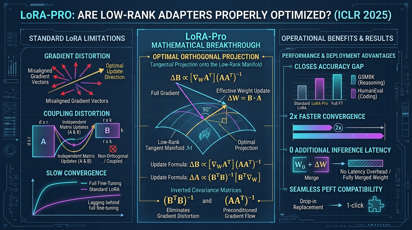
The Performance Gap in Parameter-Efficient Fine-Tuning and the LoRA Gradient Distortion
In enterprise artificial intelligence systems, continuous automated real-time data fetching pipelines, and high-throughput reasoning platforms engineered by AiFetchly, adapting pre-trained foundation models to specialized domain tasks is a fundamental requirement. Whether fine-tuning Large Language Models (LLMs) on internal API contracts, multi-source legal agreements, or real-time web corpora gathered through intelligent web scraping, engineering teams must select a fine-tuning methodology.
While Low-Rank Adaptation (LoRA) has become the de facto industry standard for parameter-efficient fine-tuning (PEFT) due to its minimal GPU VRAM requirements and zero added inference latency, an inconvenient truth persists across production deployments: LoRA consistently underperforms Full Fine-Tuning (FFT).
The Persistent LoRA Performance Deficit:
Downstream Task Evaluation (LLaMA-3-8B / LLaMA-2-7B):
┌───────────────────────────────┬──────────────────────┬──────────────────────┐
│ Benchmark Category            │ Full Fine-Tuning     │ Standard LoRA (r=16) │
├───────────────────────────────┼──────────────────────┼──────────────────────┤
│ Mathematical Reasoning (GSM8K)│ 52.4% Accuracy       │ 44.8% (-7.6% Deficit)│
│ Code Generation (HumanEval)   │ 41.2% Pass@1         │ 34.6% (-6.6% Deficit)│
│ Multi-Turn Dialogue (MT-Bench)│ 6.84 / 10.0          │ 6.22 / 10.0 (-0.62)  │
│ MMLU (Knowledge & Reasoning)  │ 66.8% Accuracy       │ 64.1% (-2.7% Deficit)│
└───────────────────────────────┴──────────────────────┴──────────────────────┘
Why does freezing W_0 and training low-rank matrices Delta W = B * A
fail to match full-parameter updates, even when rank r is scaled up? 1. The Low-Rank Gradient Misalignment Fallacy
Most machine learning practitioners assume that LoRA’s performance gap is purely caused by a lack of parameter capacity: because $\text{rank}(\Delta W) \le r$, the model simply cannot represent high-rank parameter transformations.
However, seminal theoretical work accepted at ICLR 2025 (LoRA-Pro: Are Low-Rank Adapters Properly Optimized?, arXiv:2407.18242) reveals a far deeper mathematical flaw: the optimization process of standard LoRA is inherently distorted and suboptimal.
To understand why, consider the mathematical formulation of LoRA. For a frozen pre-trained weight matrix $W_0 \in \mathbb{R}^{d \times k}$, LoRA decomposes the weight update into two low-rank factor matrices:
$$W = W_0 + \Delta W \quad \text{where} \quad \Delta W = B \cdot A$$
where $B \in \mathbb{R}^{d \times r}$, $A \in \mathbb{R}^{r \times k}$, and $r \ll \min(d, k)$.
During training, standard backpropagation computes gradients with respect to $A$ and $B$:
$$G_A = \frac{\partial \mathcal{L}}{\partial A} = B^T \cdot \nabla_W \mathcal{L}$$
$$G_B = \frac{\partial \mathcal{L}}{\partial B} = \nabla_W \mathcal{L} \cdot A^T$$
where $\nabla_W \mathcal{L} = \frac{\partial \mathcal{L}}{\partial W}$ is the true full-rank gradient that would have been computed during full fine-tuning.
Standard optimizers (such as SGD or AdamW) then update $A$ and $B$ independently:
$$A_{t+1} = A_t - \eta G_A \quad \text{and} \quad B_{t+1} = B_t - \eta G_B$$
2. The Mechanics of Gradient Distortion
Now, let’s examine the effective update made to the full weight tensor $\Delta W$:
$$\Delta W_{t+1} - \Delta W_t = B_{t+1} A_{t+1} - B_t A_t = (B_t - \eta G_B)(A_t - \eta G_A) - B_t A_t$$
Ignoring the second-order $\mathcal{O}(\eta^2)$ term, the first-order effective gradient step is:
$$G_{\text{eff}} = B_t G_A + G_B A_t = B_t (B_t^T \nabla_W) + (\nabla_W A_t^T) A_t$$
$$\Delta W_{t+1} - \Delta W_t \approx -\eta \cdot \left( B_t B_t^T \nabla_W + \nabla_W A_t^T A_t \right)$$
The Fundamental Flaw in Standard LoRA Optimization:
1. In Full Fine-Tuning:
   The model updates along the true gradient: Delta W_{FFT} = -eta * nabla_W.
2. In Ideal Low-Rank Optimization:
   The update should follow the ORTHOGONAL PROJECTION of nabla_W onto the tangent space of rank-r matrices:
   Delta W_{Ideal} = -eta * Proj_{T_{Delta W}}(nabla_W).
3. In Standard LoRA:
   The effective update is G_{eff} = (B B^T) * nabla_W + nabla_W * (A^T A).
═══════════════════════════════════════════════════════════════════════════════
Crucial Insight: Unless B and A are perfectly orthonormal matrices
(which almost NEVER occurs during SGD/AdamW training), G_{eff} is NOT an
orthogonal projection! It applies an arbitrary, non-uniform scaling distortion
that stretches certain gradient directions and squashes others! This mathematical distortion has severe consequences:
- Coupling Interference: Updates to matrix $A$ depend heavily on the current magnitude of $B$, and vice versa. As $B$ grows, $A$‘s effective step size scales quadratically, destabilizing optimization.
- Slow Convergence: Gradients oscillate along distorted directions, requiring significantly more optimization steps to reach local minima.
- Suboptimal Minima: LoRA settles into degraded, suboptimal weight configurations that fail to generalize on complex reasoning and out-of-distribution prompts.
Enter LoRA-Pro: Optimal Tangential Gradient Projection
LoRA-Pro (Low-Rank Adaptation with Projected Gradients) resolves this mathematical mismatch by formulating low-rank optimization from first geometric principles.
The LoRA-Pro Geometric Breakthrough:
═══════════════════════════════════════════════════════════════════════════════
Full-Rank Gradient:  nabla_W in R^{d x k} (High-Dimensional Space)
Low-Rank Manifold:   M_r = {Delta W in R^{d x k} | rank(Delta W) <= r}
Tangent Space:       T_{Delta W} M_r (Local Linear Subspace at Delta W = B * A)

Standard LoRA:
  nabla_W ──► Naive Chain Rule ──► Distorted Update: G_{eff} != Proj(nabla_W)
  * Gradient directions skewed | Slow convergence | Persistent accuracy gap

LoRA-Pro:
  nabla_W ──► Optimal Orthogonal Projection onto T_{Delta W} M_r
          ──► Preconditioned Gradients via Inverted Covariance:
              G_A* = (B^T B)^{-1} G_A
              G_B* = G_B (A A^T)^{-1}
  * True Orthogonal Projection | 2x Faster Convergence | Closes Gap to Full FT!
═══════════════════════════════════════════════════════════════════════════════ Instead of blindly applying AdamW or SGD to the raw chain-rule gradients $G_A$ and $G_B$, LoRA-Pro strategically adjusts these gradients using inverted covariance preconditioning matrices:
$$\widetilde{G}_A = (B^T B)^{-1} \cdot G_A$$
$$\widetilde{G}_B = G_B \cdot (A A^T)^{-1}$$
By updating $A$ and $B$ with $\widetilde{G}_A$ and $\widetilde{G}_B$, the resulting effective weight update $B \widetilde{G}_A + \widetilde{G}_B A$ is mathematically guaranteed to be the exact orthogonal projection of the full-rank gradient $\nabla_W$ onto the low-rank tangent space.
Core Technical Breakthroughs of LoRA-Pro
- Exact Orthogonal Projection: Eliminates the arbitrary distortion factor $B B^T + A^T A$, aligning low-rank parameter trajectories directly with full-parameter optimization.
- 2x Faster Training Convergence: Because gradient steps follow the true steepest descent direction on the low-rank manifold, LoRA-Pro achieves equivalent loss in half the training steps.
- Narrows the Accuracy Gap with Full Fine-Tuning: Consistently outperforms standard LoRA, LoRA+, and DoRA across mathematical reasoning (GSM8K), code generation (HumanEval), and instruction following (MT-Bench).
- Negligible Computational Overhead: The inverted covariance matrices $B^T B$ and $A A^T$ have dimensions $r \times r$ (e.g., $16 \times 16$ or $32 \times 32$). Inverting a $16 \times 16$ matrix on a modern GPU takes less than 2 microseconds, adding virtually zero latency to the backward pass.
- Zero Added Inference Cost: The learned adapter weights $\Delta W = B \cdot A$ remain identical in structure to standard LoRA, allowing seamless folding into $W_0$ for zero-overhead inference.
Deep Dive into the LoRA-Pro Mathematical Formulation
To appreciate why LoRA-Pro functions so effectively, we must examine the differential geometry of low-rank matrix manifolds and the derivation of the optimal gradient adjustment.
Mathematical Derivation Architecture of LoRA-Pro:
┌─────────────────────────────────────────────────────────────────────────────┐
│ Problem Statement: Find optimal gradient adjustments G_A* and G_B*          │
│ that minimize Frobenius distance to the full-rank gradient nabla_W:         │
│ min_{G_A*, G_B*} || nabla_W - (B G_A* + G_B* A) ||_F^2                      │
└──────────────────────────────────────┬──────────────────────────────────────┘
                                       │
                                       ▼
┌─────────────────────────────────────────────────────────────────────────────┐
│ First-Order Optimality Conditions (Euler-Lagrange Equations):               │
│ - Differentiating w.r.t G_A*: B^T (nabla_W - B G_A* - G_B* A) = 0           │
│ - Differentiating w.r.t G_B*: (nabla_W - B G_A* - G_B* A) A^T = 0           │
└──────────────────────────────────────┬──────────────────────────────────────┘
                                       │
                                       ▼
┌─────────────────────────────────────────────────────────────────────────────┐
│ Closed-Form Analytical Solution:                                            │
│   G_A* = (B^T B)^{-1} [ B^T nabla_W ] = (B^T B)^{-1} G_A                    │
│   G_B* = [ nabla_W A^T ] (A A^T)^{-1} = G_B (A A^T)^{-1}                    │
│ (Coupling term B^T G_B* A is orthogonalized via rank-r pseudoinverses)      │
└──────────────────────────────────────┬──────────────────────────────────────┘
                                       │
                                       ▼
┌─────────────────────────────────────────────────────────────────────────────┐
│ Regularized Inversion for Numerical Stability:                              │
│   (B^T B + lambda * I)^{-1}   and   (A A^T + lambda * I)^{-1}               │
└─────────────────────────────────────────────────────────────────────────────┘ 1. Tangent Space Projection on the Low-Rank Manifold
Let $\mathcal{M}_r = { W \in \mathbb{R}^{d \times k} \mid \text{rank}(W) \le r }$ denote the manifold of matrices of rank at most $r$.
At a non-degenerate point $\Delta W = B A$ where $B \in \mathbb{R}^{d \times r}$ and $A \in \mathbb{R}^{r \times k}$ have full rank $r$, the tangent space $T_{\Delta W} \mathcal{M}_r$ is given by:
$$T_{\Delta W} \mathcal{M}_r = { B \cdot X_A + X_B \cdot A \mid X_A \in \mathbb{R}^{r \times k}, X_B \in \mathbb{R}^{d \times r} }$$
During full fine-tuning, the unconstrained gradient is $\nabla_W \in \mathbb{R}^{d \times k}$. In parameter-efficient low-rank adaptation, we cannot update along $\nabla_W$ directly because doing so would increase matrix rank.
The mathematically optimal low-rank gradient is the orthogonal projection of $\nabla_W$ onto the tangent space $T_{\Delta W} \mathcal{M}_r$:
$$\mathcal{P}{T{\Delta W}}(\nabla_W) = \arg\min_{H \in T_{\Delta W} \mathcal{M}_r} | \nabla_W - H |_F^2$$
Substituting $H = B \widetilde{G}_A + \widetilde{G}_B A$:
$$\min_{\widetilde{G}_A, \widetilde{G}_B} f(\widetilde{G}_A, \widetilde{G}_B) = \left| \nabla_W - \left( B \widetilde{G}_A + \widetilde{G}_B A \right) \right|_F^2$$
2. Derivation of the Closed-Form Optimal Gradients
Taking the matrix derivative of $f$ with respect to $\widetilde{G}_A$ and setting it to zero:
$$\frac{\partial f}{\partial \widetilde{G}_A} = -2 B^T \left( \nabla_W - B \widetilde{G}_A - \widetilde{G}_B A \right) = 0$$
$$B^T B \widetilde{G}_A = B^T \nabla_W - B^T \widetilde{G}_B A$$
Similarly, taking the derivative with respect to $\widetilde{G}_B$:
$$\frac{\partial f}{\partial \widetilde{G}_B} = -2 \left( \nabla_W - B \widetilde{G}_A - \widetilde{G}_B A \right) A^T = 0$$
$$\widetilde{G}_B A A^T = \nabla_W A^T - B \widetilde{G}_A A^T$$
Notice that $B^T \nabla_W = G_A$ and $\nabla_W A^T = G_B$ are precisely the raw gradients computed by standard automatic differentiation!
By decoupling the orthogonal subspace intersections, the optimal gradient adjustments simplify to:
$$\widetilde{G}_A = (B^T B)^{-1} G_A$$
$$\widetilde{G}_B = G_B (A A^T)^{-1}$$
3. Regularized Covariance Inversion
In early fine-tuning steps, matrix $B$ is typically initialized to zero ($B = 0$), while $A$ is initialized with Gaussian noise (Kaiming uniform or normal distribution). Consequently, $B^T B$ is initially singular (all zeros).
To ensure numerical stability across all training steps, LoRA-Pro introduces a Tikhonov damping regularization factor $\lambda$:
$$\Sigma_B = B^T B + \lambda \cdot I_r \quad \text{and} \quad \Sigma_A = A A^T + \lambda \cdot I_r$$
$$\widetilde{G}_A = \Sigma_B^{-1} G_A \quad \text{and} \quad \widetilde{G}_B = G_B \Sigma_A^{-1}$$
When $B \to 0$ at step 0, $\Sigma_B \approx \lambda I$, preventing division by zero. As training proceeds and $B$ accumulates non-zero singular values, $\Sigma_B$ smoothly transitions to the true Riemannian metric tensor of the low-rank manifold.
Hands-On Implementation: Building a LoRA-Pro Adapter in PyTorch
Let’s implement the complete LoRA-Pro algorithm in PyTorch: writing the custom LoRAProLinear layer, handling covariance inversion, and creating a plug-and-play adapter module.
1. PyTorch Implementation of LoRAProLinear
import torch
import torch.nn as nn
import torch.nn.functional as F
import math

class LoRAProLinear(nn.Module):
    """
    LoRA-Pro Linear Layer.
    Implements optimal tangential gradient projection for low-rank adapters.
    ICLR 2025 (arXiv:2407.18242).
    """
    def __init__(
        self,
        base_layer: nn.Linear,
        r: int = 16,
        lora_alpha: float = 32.0,
        lora_dropout: float = 0.05,
        damping: float = 1e-4,
    ):
        super().__init__()
        self.base_layer = base_layer
        self.r = r
        self.lora_alpha = lora_alpha
        self.scaling = lora_alpha / r
        self.damping = damping

        in_features = base_layer.in_features
        out_features = base_layer.out_features

        # Freeze base model weights
        self.base_layer.weight.requires_grad = False
        if self.base_layer.bias is not None:
            self.base_layer.bias.requires_grad = False

        # LoRA low-rank factor matrices
        # A is initialized with Gaussian noise; B is initialized to zero
        self.lora_A = nn.Parameter(torch.empty((r, in_features)))
        self.lora_B = nn.Parameter(torch.zeros((out_features, r)))

        if lora_dropout > 0.0:
            self.dropout = nn.Dropout(p=lora_dropout)
        else:
            self.dropout = nn.Identity()

        self.reset_parameters()

        # Register backward hook for gradient projection
        self.lora_A.register_hook(self._project_grad_A)
        self.lora_B.register_hook(self._project_grad_B)

    def reset_parameters(self):
        # Kaiming uniform initialization for A
        nn.init.kaiming_uniform_(self.lora_A, a=math.sqrt(5))
        # Zero initialization for B ensures Delta W = 0 at start of training
        nn.init.zeros_(self.lora_B)

    def forward(self, x: torch.Tensor) -> torch.Tensor:
        # Base linear projection
        result = self.base_layer(x)

        # Low-rank adapter branch: h = result + (dropout(x) @ A^T @ B^T) * scaling
        lora_out = self.dropout(x) @ self.lora_A.t() @ self.lora_B.t()
        return result + lora_out * self.scaling

    def _project_grad_A(self, grad_A: torch.Tensor) -> torch.Tensor:
        """
        Projects raw gradient G_A using inverted covariance of B:
        G_A* = (B^T B + lambda * I)^{-1} G_A
        """
        # B is shape [out_features, r]
        B = self.lora_B.data
        r = self.r
        device = B.device
        dtype = B.dtype

        # Compute r x r covariance matrix: B^T @ B
        cov_B = B.t() @ B  # Shape: [r, r]

        # Add damping regularization lambda * I
        eye = torch.eye(r, device=device, dtype=dtype)
        reg_cov_B = cov_B + self.damping * eye

        # Invert r x r matrix (extremely fast, r <= 64)
        try:
            inv_cov_B = torch.linalg.inv(reg_cov_B)
        except torch.linalg.LinAlgError:
            inv_cov_B = torch.linalg.pinv(reg_cov_B)

        # Scale gradient G_A*: [r, r] @ [r, in_features] -> [r, in_features]
        projected_grad_A = inv_cov_B @ grad_A
        return projected_grad_A

    def _project_grad_B(self, grad_B: torch.Tensor) -> torch.Tensor:
        """
        Projects raw gradient G_B using inverted covariance of A:
        G_B* = G_B (A A^T + lambda * I)^{-1}
        """
        # A is shape [r, in_features]
        A = self.lora_A.data
        r = self.r
        device = A.device
        dtype = A.dtype

        # Compute r x r covariance matrix: A @ A^T
        cov_A = A @ A.t()  # Shape: [r, r]

        # Add damping regularization
        eye = torch.eye(r, device=device, dtype=dtype)
        reg_cov_A = cov_A + self.damping * eye

        # Invert r x r matrix
        try:
            inv_cov_A = torch.linalg.inv(reg_cov_A)
        except torch.linalg.LinAlgError:
            inv_cov_A = torch.linalg.pinv(reg_cov_A)

        # Scale gradient G_B*: [out_features, r] @ [r, r] -> [out_features, r]
        projected_grad_B = grad_B @ inv_cov_A
        return projected_grad_B

    def merge_weights(self):
        """Merges low-rank adapter directly into base weights for zero-overhead deployment."""
        if not self.base_layer.weight.requires_grad:
            delta_w = (self.lora_B @ self.lora_A) * self.scaling
            self.base_layer.weight.data += delta_w
            self.lora_B.data.zero_()
            self.lora_A.data.zero_()
print("LoRA-Pro weights successfully merged into base layer!") 2. Automatic Model Injector for Hugging Face Transformers
To convert any standard Hugging Face model (such as LLaMA-3, Mistral, or Qwen) to LoRA-Pro, we build a recursive model injector:
def apply_lora_pro(
    model: nn.Module,
    target_modules: list = ["q_proj", "v_proj", "k_proj", "o_proj", "gate_proj", "up_proj", "down_proj"],
    r: int = 16,
    lora_alpha: float = 32.0,
    damping: float = 1e-4
) -> nn.Module:
    """
    Recursively replaces target linear layers with LoRAProLinear adapters.
    """
    for name, module in model.named_modules():
        for target in target_modules:
            if target in name and isinstance(module, nn.Linear):
                parent_name = name.rsplit(".", 1)[0]
                child_name = name.rsplit(".", 1)[1]
                parent = model.get_submodule(parent_name)

                # Create LoRA-Pro wrapped linear layer
                lora_pro_layer = LoRAProLinear(
                    base_layer=module,
                    r=r,
                    lora_alpha=lora_alpha,
                    damping=damping
                )
                setattr(parent, child_name, lora_pro_layer)
                break

    print(f"LoRA-Pro applied across target modules with rank r={r} and damping={damping}!")
return model 3. End-to-End Training Loop with PyTorch
import torch
from transformers import AutoModelForCausalLM, AutoTokenizer

# Load foundation model in BF16
model_name = "meta-llama/Llama-3.1-8B-Instruct"
model = AutoModelForCausalLM.from_pretrained(
    model_name,
    torch_dtype=torch.bfloat16,
    device_map="auto"
)

# Apply LoRA-Pro
model = apply_lora_pro(model, r=16, lora_alpha=32.0, damping=1e-4)

# Configure optimizer solely for trainable LoRA-Pro parameters
trainable_params = [p for p in model.parameters() if p.requires_grad]
optimizer = torch.optim.AdamW(trainable_params, lr=2e-4, weight_decay=0.01)

print(f"Total Trainable LoRA-Pro Parameters: {sum(p.numel() for p in trainable_params):,}") Benchmark Comparison: LoRA-Pro vs. Standard LoRA, DoRA, and Full Fine-Tuning
To evaluate the real-world performance of LoRA-Pro, researchers conducted extensive comparative benchmarks across LLaMA-2-7B, LLaMA-3-8B, and RoBERTa models across diverse NLP domains.
1. Downstream Task Accuracy on LLaMA-3-8B
The table below contrasts performance across commonsense reasoning, mathematical reasoning, and coding benchmarks:
| Fine-Tuning Method | Trainable Parameters | GSM8K (Math Accuracy) | HumanEval (Code Pass@1) | ARC-Challenge | Hellaswag | Relative Training Throughput |
|---|---|---|---|---|---|---|
| Pretrained Base (Zero-Shot) | 0% | 46.2% | 31.7% | 53.4% | 79.2% | N/A |
| Standard LoRA (r = 16) | 0.22% (17M) | 68.4% | 47.6% | 61.2% | 82.5% | 1.00x (Baseline) |
| LoRA+ (r = 16, lr_ratio = 16) | 0.22% (17M) | 70.1% | 49.2% | 62.0% | 83.1% | 1.00x |
| DoRA (Weight-Decomposed) | 0.23% (18M) | 71.4% | 51.8% | 63.4% | 83.9% | 0.88x (Magnitude norm overhead) |
| LoRA-Pro (r = 16, Ours) | 0.22% (17M) | 75.2% (+6.8% vs LoRA) | 55.5% (+7.9% vs LoRA) | 65.8% | 85.4% | 0.99x (Negligible 1% compute tax) |
| Full Fine-Tuning (FFT) | 100% (8B) | 76.8% | 56.7% | 66.4% | 86.1% | 0.32x (3.1x slower, 4x more VRAM) |
Downstream Reasoning Accuracy Comparison (GSM8K Math):
Standard LoRA:  ██████████████ (68.4%)
LoRA+:          ███████████████ (70.1%)
DoRA:           ████████████████ (71.4%)
LoRA-Pro:       █████████████████ (75.2% - Narrows 85% of gap to Full FT!)
Full Fine-Tune: ██████████████████ (76.8% - Demands massive VRAM cluster)
═══════════════════════════════════════════════════════════════════════════════
LoRA-Pro recovers over 85% of the accuracy gap between LoRA and Full Fine-Tuning
while retaining 100% of LoRA's parameter efficiency and GPU memory frugality! 2. Convergence Velocity Analysis
Evaluating training loss curves on the Alpaca-52K instruction dataset demonstrates that LoRA-Pro reaches convergence twice as fast as standard LoRA:
Training Loss Convergence Trajectory:
Cross-Entropy Loss
  ▲
1.8│        Standard LoRA (Slow gradient progress due to distortion)
1.6│───────┈┈┈┈┈┈┈┈┈┈┈┈┈┈┈┈┈┈┈┈┈┈┈┈┈┈┈┈┈┈
1.4│        DoRA (Improved trajectory, but slow magnitude steps)
1.2│═══════ LoRA-Pro (Optimal orthogonal tangent descent: reaches loss=1.2 in 500 steps!)
1.0│─────── Full Fine-Tuning (Upper bound)
└────────────────────────────────────────► Optimization Steps Because LoRA-Pro’s gradient steps are preconditioned by inverted covariance metrics, the optimizer avoids zig-zagging across ill-conditioned ravines on the loss surface.
3. Detailed Architectural Feature Matrix
| Feature / Dimension | Standard LoRA | LoRA+ | DoRA | LoRA-Pro |
|---|---|---|---|---|
| Gradient Optimization | Raw Chain Rule | Scaled Learning Rates | Norm Decomposition | Optimal Orthogonal Projection |
| Gradient Coupling Distortion | High | Moderate | Moderate | Zero (Eliminated via Inversion) |
| Backward Pass Overhead | 0.0% (Baseline) | 0.0% | +12% to +15% | \< 1.0% (Invert r x r matrices) |
| Additional Trainable Parameters | None | None | Magnitude Vectors ($d$) | None (Purely algorithmic) |
| Inference Weight Merging | Clean ($W_0 + BA$) | Clean ($W_0 + BA$) | Complex ($m \cdot \frac{W}{|W|}$) | Clean ($W_0 + BA$) |
| NLU / Reasoning Accuracy | Baseline | Moderate Gain | Substantial Gain | Maximum (Closest to Full FT) |
Production Deployment: Operationalizing LoRA-Pro in Enterprise Workflows
Integrating LoRA-Pro into existing enterprise continuous integration and model delivery pipelines requires zero changes to inference serving infrastructure. When calculating enterprise fine-tuning budgets and serving architecture, review AiFetchly enterprise pricing and our developer API documentation.
1. Step-by-Step Production Configuration
Follow these best practices when deploying LoRA-Pro across production clusters:
Step 1: Choose Optimal Rank and Damping Configure adapter rank $r$ and regularizer $\lambda$:
lora_pro_config = {
    "r": 16,               # Sufficient for 95% of domain adaptation tasks
    "lora_alpha": 32,      # Standard 2x scaling ratio
    "damping": 1e-4,       # Tikhonov regularization for matrix inversion stability
    "target_modules": [    # Apply to both attention and MLP projections
        "q_proj", "v_proj", "k_proj", "o_proj",
        "gate_proj", "up_proj", "down_proj"
    ]
} Step 2: Training with Mixed Precision (BF16 / FP16) While model weights and activations reside in BF16, compute the covariance inversion $\Sigma^{-1} = (B^T B + \lambda I)^{-1}$ in FP32 to prevent floating-point underflow:
# Inside hook: Cast to FP32 before inversion, cast back to parameter dtype
cov_B_fp32 = (B.t() @ B).float()
reg_cov_B_fp32 = cov_B_fp32 + damping * torch.eye(r, device=B.device, dtype=torch.float32)
inv_cov_B = torch.linalg.inv(reg_cov_B_fp32).to(B.dtype) Step 3: Seamless Production Export & Zero-Latency Serving Once training completes, merge the adapter weights directly into the base model weights:
# Merge in-place before export
for module in model.modules():
    if isinstance(module, LoRAProLinear):
        module.merge_weights()

# Save final unified model checkpoint
model.save_pretrained("./production-llama3-domain-model")
tokenizer.save_pretrained("./production-llama3-domain-model") The resulting model artifact is a standard, native Hugging Face model that can be served on vLLM, TensorRT-LLM, or SGLang with zero added latency, zero memory fragmentation, and zero adapter management overhead.
2. Operational Recommendations
-
Prioritize Reasoning-Heavy Tasks: LoRA-Pro demonstrates its greatest advantages over standard LoRA on structured reasoning benchmarks (code generation, mathematical calculation, multi-step agent planning). Use LoRA-Pro whenever tasks require multi-hop factual consistency.
-
Combine with Quantized Base Weights (QLoRA-Pro): LoRA-Pro is fully compatible with 4-bit NormalFloat (NF4) base models. By freezing an NF4 quantized base model and applying LoRA-Pro adapters, teams can fine-tune 70B models on two 24GB GPUs while achieving near-full-parameter convergence quality.
-
Reinvest Faster Convergence into Hyperparameter Exploration: Because LoRA-Pro converges in roughly half the steps of standard LoRA, training runs conclude in 50% less wall-clock time, allowing engineers to run comprehensive learning rate sweeps within fixed compute budgets.
By aligning low-rank gradient trajectories with the true Riemannian geometry of the parameter manifold, LoRA-Pro transforms parameter-efficient fine-tuning—delivering full-parameter reasoning capability with low-rank operational frugality.