LoRA Guide: Low-Rank Adaptation & PEFT Architecture
The Problem: The Computational and Storage Crisis of Full Fine-Tuning
In modern enterprise machine learning, autonomous agent development, and high-precision data extraction platforms like AiFetchly, adapting general-purpose foundation models (such as LLaMA-3, Mistral, or Qwen) to specialized downstream tasks is a daily engineering requirement.
Historically, the standard approach was Full Fine-Tuning (FFT): taking a pre-trained model and updating all of its dense weight matrices via standard backpropagation.
While full fine-tuning maximizes expressive power, scaling this approach across modern multi-billion-parameter foundation models creates an unsustainable computational and operational crisis:
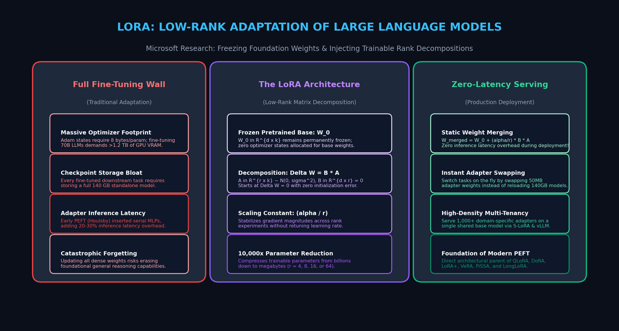
1. The Adam Optimizer VRAM Tax in Full Fine-Tuning
The primary bottleneck in full fine-tuning is not the static model weights themselves, but the massive memory footprint of the optimizer states:
- In 16-bit precision (
bfloat16orfloat16), a 70B parameter model requires 140 GB of VRAM just to hold the model parameters. - During training with the standard AdamW optimizer, each parameter requires:
- 2 bytes for the parameter weight.
- 2 bytes for the gradient.
- 4 bytes for the first momentum state ($m_t$).
- 4 bytes for the second momentum state ($v_t$).
- 4 bytes for the FP32 master weight copy to ensure numerical stability during gradient accumulation.
- Total memory per parameter reaches 16 to 18 bytes.
- For a 70B parameter model, full fine-tuning demands over 1.1 to 1.2 Terabytes of GPU High-Bandwidth Memory (HBM) solely for weights, gradients, and optimizer states—completely excluding KV caches and activation buffers.
Consequently, fine-tuning a 70B model requires expensive multi-node GPU clusters (e.g., 8x or 16x 80GB H100 GPUs) interconnected with high-bandwidth NVLink and InfiniBand fabrics.
2. Checkpoint Bloat in Multi-Task and Multi-Tenant Deployments
In real-world SaaS platforms and multi-agent systems, an organization rarely maintains just one fine-tuned model:
- An enterprise might deploy customized subagents for 500 distinct tasks: legal contract extraction, financial balance sheet parsing, medical coding, customer support routing, and SQL synthesis.
- Under full fine-tuning, every single fine-tuned task yields a full independent model checkpoint.
- Storing 500 independent 70B checkpoints requires over 70 Terabytes of disk storage.
- In serving runtimes, switching between tasks requires evicting an entire 140 GB model from GPU VRAM and reloading a new one over the PCIe bus, introducing severe multi-second latency spikes and causing GPU compute starvation.
3. The Failure of Early PEFT: Latency Overhead and Context Shrinkage
Before LoRA, researchers introduced early Parameter-Efficient Fine-Tuning (PEFT) techniques, but each introduced prohibitive operational compromises:
- Series Adapters (Houlsby et al., 2019): Inserted small two-layer feed-forward bottleneck networks sequentially after the self-attention and MLP blocks. Because these layers must be evaluated sequentially in every forward pass, they introduced a 20% to 30% inference latency overhead on modern GPUs.
- Prefix Tuning / Prompt Tuning (Li & Liang, 2021; Lester et al., 2021): Prepended trainable virtual prompt tokens to the Key and Value matrices in attention layers. While avoiding architectural modifications, prefix tokens consume valuable context window capacity, reducing the effective token budget available for long prompts and agentic tool outputs.
The industry faced a critical challenge: Can we achieve the accuracy of full fine-tuning while updating only a fraction of parameters, requiring zero extra inference latency, and enabling seamless multi-tenant serving?
The Theoretical Foundation: The Intrinsic Rank Hypothesis
To solve this dilemma, researchers at Microsoft (Edward Hu et al., ICLR 2022) introduced LoRA (Low-Rank Adaptation).
LoRA is grounded in a foundational mathematical concept established in empirical deep learning: the Intrinsic Dimension Hypothesis (Li et al., 2018; Aghajanyan et al., 2020).
1. Low-Dimensional Manifolds in Overparameterized Networks
Overparameterized neural networks contain millions or billions of parameters. However, when these networks learn representations, their internal weights do not distribute themselves randomly across the entire high-dimensional parameter space $\mathbb{R}^{D}$.
Instead, pre-trained models converge onto a remarkably low-dimensional manifold. Aghajanyan et al. (2020) demonstrated that pre-trained language models can be successfully adapted to complex downstream tasks by optimizing within a randomly projected subspace of astonishingly small intrinsic dimension $d_{ ext{int}} \ll D$.
2. Measuring Task Complexity via Intrinsic Dimension
The intrinsic dimension reflects the fundamental difficulty of the target objective:
- A base model trained on trillions of tokens already possesses vast syntactic, grammatical, and semantic knowledge.
- Adapting that model to summarize customer service transcripts or extract structured JSON tables does not require learning an entirely new world model; it merely requires shifting the model’s behavioral posture.
- Because the task-specific shift is constrained, the weight update matrix $\Delta W$ has an extremely low intrinsic rank.
3. Why Full-Rank Updates Are Redundant
In full fine-tuning, every linear layer update $\Delta W \in \mathbb{R}^{d imes k}$ is parameterized as a dense, full-rank matrix with $ ext{rank}(\Delta W) = \min(d, k)$.
For a transformer layer with hidden dimension $d = 4096$ and feed-forward dimension $k = 14336$:
- Full fine-tuning optimizes $4096 imes 14336 \approx 58.7 ext{ million parameters}$ per matrix.
- However, if the underlying task variation only spans an intrinsic rank of $r = 8$ or $r = 16$, then over 99.9% of the degrees of freedom in $\Delta W$ are redundant noise!
- LoRA capitalizes on this redundancy by enforcing a low-rank factorization directly within the network architecture.
The LoRA Architecture and Mathematical Mechanics
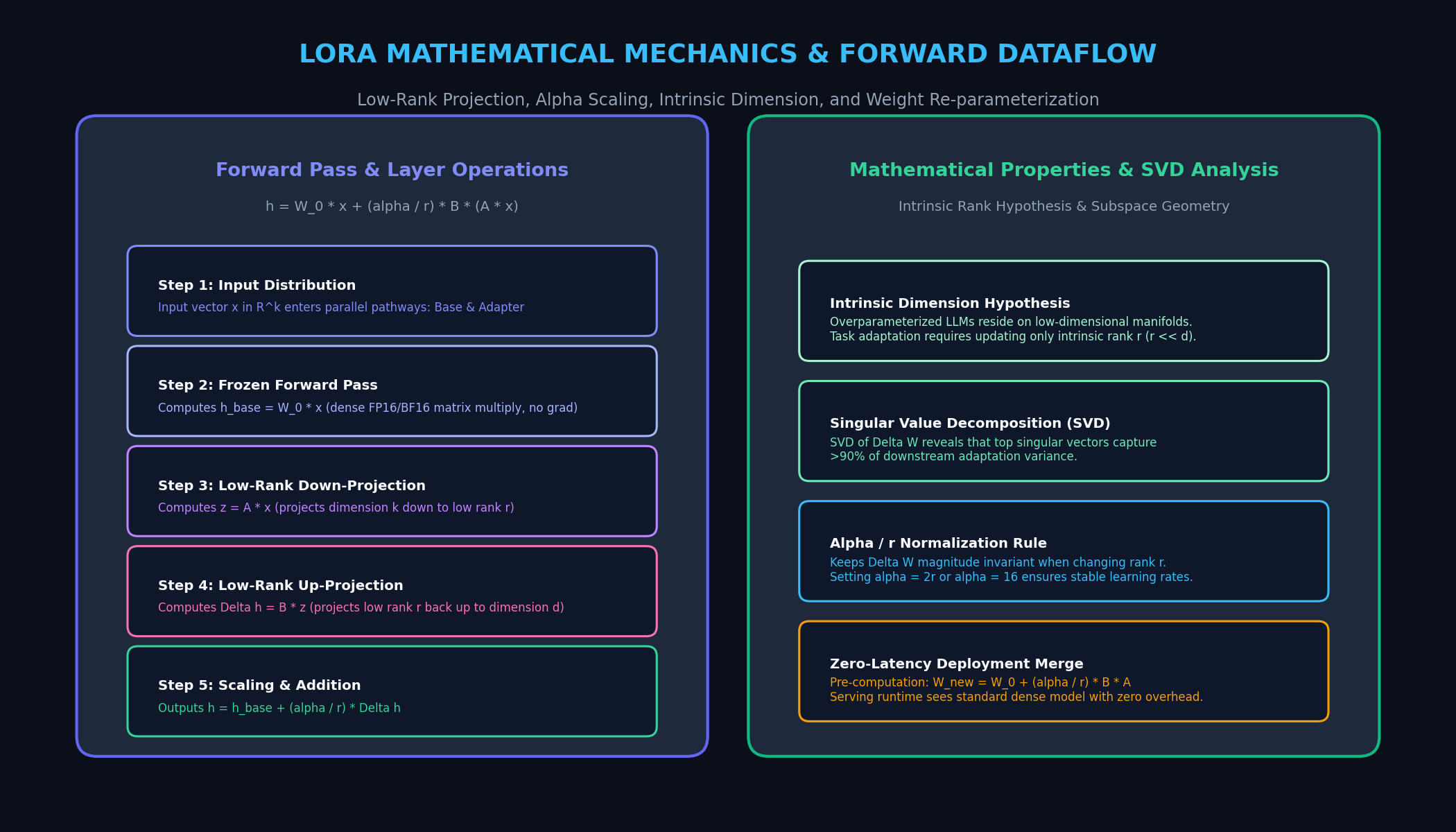
Instead of updating the full weight tensor $W_0 \in \mathbb{R}^{d imes k}$, LoRA freezes $W_0$ and parameterizes the accumulated update $\Delta W$ as the matrix product of two low-rank matrices:
$$W = W_0 + \Delta W = W_0 + \frac{\alpha}{r} (B \cdot A)$$
Where:
- $W_0 \in \mathbb{R}^{d imes k}$ represents the pre-trained base model weights, held strictly frozen throughout training.
- $B \in \mathbb{R}^{d imes r}$ is the low-rank up-projection matrix.
- $A \in \mathbb{R}^{r imes k}$ is the low-rank down-projection matrix.
- $r \ll \min(d, k)$ is the chosen rank hyperparameter (typically $r \in {4, 8, 16, 32, 64}$).
- $\alpha$ is a constant scaling hyperparameter.
1. Low-Rank Matrix Factorization: Delta W = B * A
During the forward pass, for an input token representation $x \in \mathbb{R}^{B imes T imes k}$:
$$h = W_0 x + \Delta W x = W_0 x + \frac{\alpha}{r} B (A x)$$
Observe the computational flow:
- The input $x$ is multiplied by frozen base matrix $W_0$, yielding the standard base activation $h_{ ext{base}} = W_0 x$.
- In parallel, $x$ is projected through matrix $A$, compressing the dimension from $k$ down to low rank $r$:
$$z = A x, \quad z \in \mathbb{R}^{B imes T imes r}$$
- The compressed representation $z$ is projected back up through matrix $B$, expanding the dimension from $r$ to $d$:
$$\Delta h = B z = B (A x), \quad \Delta h \in \mathbb{R}^{B imes T imes d}$$
- Both pathways are summed together with the scaling factor $\frac{\alpha}{r}$.
2. Asymmetric Initialization: Why B = 0 and A ~ N(0, sigma^2)
A crucial engineering detail of LoRA is its asymmetric weight initialization:
- Matrix A is initialized from a zero-mean Gaussian distribution $A \sim \mathcal{N}(0, \sigma^2)$ (or Kaiming uniform).
- Matrix B is initialized strictly to zero ($B = 0$).
Why is this initialization critical? At the very beginning of training (step 0):
$$\Delta W = B \cdot A = 0 \cdot A = 0$$
Because $\Delta W = 0$ at step 0, the model’s output is mathematically identical to the unadapted pre-trained base model:
$$h = W_0 x + 0 = W_0 x$$
This ensures that fine-tuning begins cleanly from the pre-trained distribution. There is no initial noise, no catastrophic early loss spikes, and no need for extensive learning rate warm-up schedules to counteract random adapter outputs.
3. The Alpha / r Scaling Factor and Gradient Normalization
In the LoRA formulation, the update is scaled by $\frac{\alpha}{r}$, where $\alpha$ is a fixed scalar constant (typically set to $\alpha = 16$ or $\alpha = 2r$).
Why include $\frac{\alpha}{r}$ rather than absorbing it into the learning rate?
- When fine-tuning, ML engineers frequently experiment with different ranks (e.g., comparing $r = 4$, $r = 16$, and $r = 64$) to identify the optimal capacity for a task.
- If the formulation were simply $B A$, increasing $r$ would linearly scale the magnitude of the gradient updates and activations, requiring practitioners to retune the learning rate and optimizer hyperparameters for every single rank trial.
- By scaling by $\frac{\alpha}{r}$, the expected magnitude of the update remains approximately invariant to changes in $r$. Once an optimal learning rate is discovered for $r = 8$, the same learning rate can be used seamlessly when scaling up to $r = 64$.
4. Which Weight Matrices to Adapt? Attention vs. Feed-Forward MLPs
In a Transformer block, linear layers appear in two distinct locations: Multi-Head Attention ($W_q, W_k, W_v, W_o$) and the Feed-Forward Network ($W_{ ext{gate}}, W_{ ext{up}}, W_{ ext{down}}$).
Hu et al. investigated which matrices yield the highest adaptation efficiency:
- Adapting Attention Only ($W_q, W_v$): The original LoRA paper prioritized adapting Query ($W_q$) and Value ($W_v$) projection matrices. Adapting both $W_q$ and $W_v$ with $r = 4$ matched the accuracy of adapting all attention matrices with $r = 8$, while keeping parameters minimal.
- Adapting All Linear Layers (Modern 2025/2026 Standard): In modern practice (including QLoRA and frontier fine-tuning pipelines), practitioners apply LoRA across all linear projection layers ($W_q, W_k, W_v, W_o$ plus MLP layers). Experiments demonstrate that adapting all linear layers with a smaller rank (e.g., $r = 8$ or $r = 16$) consistently outperforms adapting only attention layers with a larger rank (e.g., $r = 64$).
Zero-Latency Serving and Multi-Tenant Architecture
The architectural triumph of LoRA in production is its dual operating mode: lightweight during training, zero-overhead during inference.
1. Static Weight Merging: Zero Overhead at Inference Time
For single-tenant production deployments (where a dedicated model serves a specific domain), LoRA introduces zero additional latency and zero memory overhead.
Because matrix multiplication is linear and associative, the low-rank update can be folded directly into the base weights before deploying the model:
$$W_{ ext{merged}} = W_0 + \frac{\alpha}{r} (B \cdot A)$$
At deployment time:
- The engine computes the static matrix product $\Delta W = \frac{\alpha}{r} B A$.
- It adds $\Delta W$ directly to the frozen weights $W_0$.
- The adapter matrices $A$ and $B$ are deleted from memory.
The resulting model is an exact, standard Transformer model. It executes standard dense GEMM kernels on GPU Tensor Cores, utilizes standard KV caches, and runs with identically zero latency penalty compared to the base model.
If the base model needs to be updated or repurposed later, the adapter can be subtracted just as easily:
$$W_0 = W_{ ext{merged}} - \frac{\alpha}{r} (B \cdot A)$$
2. Dynamic Adapter Swapping in Multi-Tenant Environments (S-LoRA and vLLM)
In multi-tenant cloud environments (such as serving thousands of enterprise customer bots or specialized extraction scrapers), merging weights is impractical because storing thousands of 140 GB models is impossible.
Instead, modern serving engines (such as S-LoRA, Punica, and vLLM Multi-LoRA) leverage LoRA’s low-rank structure for dynamic routing:
- Unified Base Model: A single frozen copy of the 70B base model is loaded into GPU VRAM.
- Dynamic Adapter Cache: Thousands of task-specific adapter weights ($A$ and $B$, typically only 20 MB to 100 MB each) are stored in host CPU DRAM or NVMe storage.
- Batched Adapter Kernel (BMM): During batched inference, the server receives a heterogeneous batch where Request 1 uses Adapter A, Request 2 uses Adapter B, and Request 3 uses Adapter C. Specialized CUDA kernels (such as grouped GEMM or segmented gather-scatter) evaluate the shared base model in a single unified GEMM, and then apply the tiny adapter projections per request stream on the fly.
- This allows a single 8x A100 node to serve over 2,000 distinct customized enterprise LLMs simultaneously with near-zero throughput degradation.
3. SVD Analysis: Subspace Overlap Across Tasks
When performing Singular Value Decomposition (SVD) on learned LoRA updates $\Delta W = U \Sigma V^T$, fascinating mathematical properties emerge:
- The singular value spectrum $\Sigma$ decays rapidly: the top 4 singular vectors account for over 80% of the total spectral energy of the update.
- When comparing LoRA adapters trained on different tasks (e.g., legal parsing vs. code synthesis), the right singular vectors $V$ (input feature directions) exhibit significant overlap with the top singular vectors of the pre-trained base model $W_0$, indicating that LoRA selectively amplifies pre-existing latent capabilities rather than carving out arbitrary new subspaces.
4. Comparison Table: Parameter-Efficient Fine-Tuning Paradigms
The following table contrasts LoRA against historical and modern PEFT alternatives:
| Adaptation Framework | Trainable Parameter % | Added Inference Latency | GPU Memory Savings vs. FFT | Zero-Latency Merging? | Primary Trade-Off |
|---|---|---|---|---|---|
| Full Fine-Tuning (FFT) | 100% | None | 0% (Requires ~16B/param) | Inapplicable | Extreme VRAM & checkpoint storage costs |
| Houlsby Adapters | 1% – 3% | +20% to +30% (High) | ~60% | No (Sequential layers) | Severe latency penalty on GPUs |
| Prefix / Prompt Tuning | < 0.1% | Minimal | ~70% | No (Consumes context) | Shrinks available prompt context window |
| LoRA (Microsoft) | 0.01% – 0.5% | Zero (when merged) | ~65% to ~75% | Yes ($W_0 + \frac{\alpha}{r}BA$) | Universal baseline standard |
| QLoRA (Dettmers et al.) | 0.01% – 0.5% | Minimal (NF4 dequant) | ~85% (Base in 4-bit) | Yes (after dequantization) | Slight dequantization overhead in training |
| DoRA (Liu et al.) | 0.02% – 0.6% | Zero (when merged) | ~65% to ~75% | Yes | Decomposes weight magnitude and direction |
| VeRA (Kopiczko et al.) | < 0.001% | Zero (when merged) | ~90% | Yes | Frozen random matrices with scaling vectors |
End-to-End Implementation: Building a Production LoRA Module in PyTorch
To understand how LoRA operates at the tensor level, let us examine an end-to-end, runnable PyTorch implementation of the LoRALinear layer.
This implementation features linear forward execution, rank down-projection, up-projection, alpha scaling, and production weight merging/unmerging logic.
1. PyTorch Implementation of LoRALinear with Dynamic Merging
import math
import torch
import torch.nn as nn
import torch.nn.functional as F

class LoRALinear(nn.Module):
    """
    Production-grade LoRA Linear Layer.
    Wraps a frozen pre-trained linear weight W_0 and injects trainable rank decomposition matrices:
    Delta W = (alpha / r) * B * A

    Reference: Hu et al. (Microsoft, ICLR 2022)
    """
    def __init__(
        self,
        in_features: int,
        out_features: int,
        r: int = 8,
        lora_alpha: float = 16.0,
        lora_dropout: float = 0.05,
        bias: bool = False
    ):
        super().__init__()
        self.in_features = in_features
        self.out_features = out_features
        self.r = r
        self.lora_alpha = lora_alpha
        self.scaling = lora_alpha / r if r > 0 else 1.0

        # 1. Base pre-trained weight (held strictly frozen)
        self.weight = nn.Parameter(torch.empty((out_features, in_features)), requires_grad=False)
        if bias:
            self.bias = nn.Parameter(torch.empty(out_features), requires_grad=False)
        else:
            self.register_parameter('bias', None)

        # 2. Trainable LoRA low-rank matrices
        if r > 0:
            # Matrix A: Down-projection from in_features -> r
            self.lora_A = nn.Parameter(torch.empty((r, in_features)))
            # Matrix B: Up-projection from r -> out_features
            self.lora_B = nn.Parameter(torch.empty((out_features, r)))
            self.lora_dropout = nn.Dropout(p=lora_dropout) if lora_dropout > 0.0 else nn.Identity()
        else:
            self.register_parameter('lora_A', None)
            self.register_parameter('lora_B', None)
            self.lora_dropout = nn.Identity()

        # State tracking for inference weight merging
        self.merged = False

        # Initialize weights
        self.reset_parameters()

    def reset_parameters(self):
        """Initializes base weights and applies asymmetric LoRA initialization."""
        # Initialize base weight with standard Kaiming uniform
        nn.init.kaiming_uniform_(self.weight, a=math.sqrt(5))
        if self.bias is not None:
            fan_in, _ = nn.init._calculate_fan_in_and_fan_out(self.weight)
            bound = 1 / math.sqrt(fan_in) if fan_in > 0 else 0
            nn.init.uniform_(self.bias, -bound, bound)

        # Asymmetric LoRA initialization: A ~ Kaiming uniform, B = 0
        if self.r > 0:
            nn.init.kaiming_uniform_(self.lora_A, a=math.sqrt(5))
            nn.init.zeros_(self.lora_B)

    def merge_weights(self):
        """Folds Delta W into base weight W_0 for zero-latency production inference."""
        if self.r > 0 and not self.merged:
            # W_merged = W_0 + (alpha / r) * (B @ A)
            delta_w = (self.lora_B @ self.lora_A) * self.scaling
            self.weight.data.add_(delta_w)
            self.merged = True

    def unmerge_weights(self):
        """Subtracts Delta W from W_merged to recover original base weight W_0."""
        if self.r > 0 and self.merged:
            delta_w = (self.lora_B @ self.lora_A) * self.scaling
            self.weight.data.sub_(delta_w)
            self.merged = False

    def forward(self, x: torch.Tensor) -> torch.Tensor:
        """
        Forward pass.
        If weights are merged, executes standard linear transformation.
        If unmerged, computes parallel base and low-rank adapter pathways.
        """
        if self.merged or self.r == 0:
            return F.linear(x, self.weight, self.bias)

        # 1. Base frozen forward pass: h_base = x @ W_0^T
        base_out = F.linear(x, self.weight, self.bias)

        # 2. LoRA adapter forward pass: Delta h = (dropout(x) @ A^T) @ B^T * scaling
        # Down-projection: (batch, seq_len, in_features) -> (batch, seq_len, r)
        dropped_x = self.lora_dropout(x)
        low_rank_z = F.linear(dropped_x, self.lora_A)

        # Up-projection: (batch, seq_len, r) -> (batch, seq_len, out_features)
        adapter_out = F.linear(low_rank_z, self.lora_B) * self.scaling

        # 3. Sum parallel representations
return base_out + adapter_out Empirical Benchmarks: LoRA vs. Full Fine-Tuning Across Model Scales
The empirical validation presented by Microsoft Research proved that parameter-efficient low-rank adaptation matches or even exceeds the performance of full fine-tuning.
1. GLUE, WikiSQL, and GSM8K Task Performance
Across standardized NLP benchmarks evaluated on RoBERTa-large, DeBERTa-XXL, and GPT-3 (175B):
| Model & Task | Adaptation Method | Trainable Params | GLUE Score / Accuracy | WikiSQL (Logical Form) | GSM8K (Math Reasoning) |
|---|---|---|---|---|---|
| RoBERTa-Large (355M) | Full Fine-Tuning (FFT) | 355.0M (100%) | 88.9 | 86.4% | - |
| RoBERTa-Large | Houlsby Adapters ($d_m=64$) | 3.0M (0.8%) | 87.2 | 85.1% | - |
| RoBERTa-Large | Prefix Tuning ($l_p=20$) | 0.8M (0.2%) | 87.4 | 85.8% | - |
| RoBERTa-Large | LoRA ($r=8, W_q, W_v$) | 0.8M (0.2%) | 89.3 (+0.4) | 86.8% (+0.4%) | - |
| GPT-3 (175 Billion) | Full Fine-Tuning (FFT) | 175.0B (100%) | 89.6 | 73.8% | 34.0% |
| GPT-3 (175 Billion) | LoRA ($r=4, W_q, W_v$) | 4.7M (0.002%) | 90.0 (+0.4) | 74.4% (+0.6%) | 35.2% (+1.2%) |
Key insights from empirical benchmarks:
- LoRA Outperforms Full Fine-Tuning: On both RoBERTa and GPT-3, LoRA achieved higher task accuracy than full fine-tuning while training over 10,000 times fewer parameters. By constraining updates to low-rank subspaces, LoRA acts as an implicit regularizer, preventing the model from overfitting on small downstream datasets.
- Superior Sample Efficiency: LoRA stabilizes optimization on small target datasets where full fine-tuning frequently exhibits representation collapse.
2. Training VRAM Savings and Throughput Benchmarks
During training across standard NVIDIA hardware:
Training VRAM Usage for 70B LLM Fine-Tuning (Batch Size = 4)
----------------------------------------------------------------------
Full Fine-Tuning (FFT)  | ======================================= (>1,200 GB)
LoRA (BF16 Base, r=16)  | ================== (~380 GB)  <-- 3x VRAM Reduction!
QLoRA (4-Bit Base, r=16)| ======= (~48 GB) <-- Single 80GB GPU! - 3x VRAM Reduction: Because optimizer states are only maintained for $A$ and $B$, static VRAM during training is cut by over 65% on BF16 base models.
- Single-GPU Feasibility: When combined with 4-bit NormalFloat base quantization (QLoRA), 70B parameter models can be fine-tuned on a single 80GB A100 GPU, democratizing cutting-edge model adaptation for teams worldwide.
Strategic Engineering Guide: Deploying LoRA in 2026 Production Pipelines
For ML practitioners, AI systems engineers, and developers building autonomous extraction agents like AiFetchly, deploying LoRA in production pipelines requires understanding three fundamental best practices:
1. Choosing the Optimal Rank (r) and Alpha for Domain Adaptation
- Narrow Syntax Tasks ($r = 4$ to $r = 8$): When adapting an LLM for structured output formatting, SQL query translation, or HTML entity extraction, the intrinsic dimension is low. Use $r = 8$ and $\alpha = 16$. Increasing rank beyond 8 on narrow formatting tasks increases training time without improving task accuracy.
- Complex Domain Knowledge ($r = 32$ to $r = 64$): When fine-tuning on complex domains (such as medical diagnosis, legal jurisprudence, or proprietary enterprise documentation), the model must absorb rich semantic associations. Use $r = 32$ or $r = 64$ with $\alpha = 64$ applied across all linear layers.
- The Alpha Rule: Always maintain $\alpha = 2 imes r$ (or a fixed $\alpha = 16$) as a standard baseline to ensure stable gradient propagation.
2. Combining LoRA with Quantization (QLoRA and 4-Bit Substrates)
When memory is constrained:
- Load the base model in 4-bit NormalFloat (
NF4) usingbitsandbytesor native FP4 microscaling on NVIDIA Blackwell hardware. - Attach unquantized
bfloat16LoRA adapters to all attention and MLP projection layers. - Compute forward activations by dynamically dequantizing base weights into 16-bit registers, performing matrix multiplications, and updating only the 16-bit adapter gradients.
3. Fine-Tuning Autonomous Data Extraction and Web Agents
In agentic data extraction pipelines:
- Train separate, specialized LoRA adapters for distinct agent sub-tasks (e.g., one adapter for DOM tree parsing, one adapter for API schema translation, and one adapter for error diagnosis).
- Store these adapters in a shared S-LoRA dynamic cache.
- During runtime, route requests to the appropriate adapter dynamically without incurring model reloading penalties.
By parameterizing weight updates as low-rank decompositions and enabling zero-latency production serving, LoRA remains the foundational bedrock of parameter-efficient deep learning in 2026.