LoRA-GA Guide: Gradient Approximation for Faster LLMs
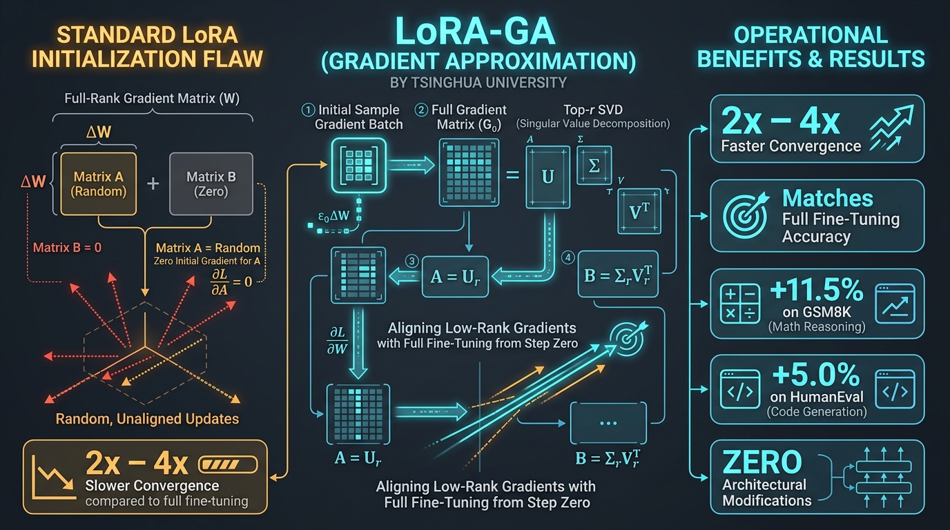
The Initialization Flaw in Low-Rank Adaptation and the Convergence Tax
In modern enterprise machine learning systems, autonomous agent workflows, and real-time knowledge discovery pipelines powered by AiFetchly, adapting Large Language Models (LLMs) to specialized downstream tasks is a constant requirement. Whether training models on newly scraped documentation through resilient web scraping interfaces or continuous temporal data ingested via automated data fetching pipelines, parameter-efficient fine-tuning (PEFT) has become the default deployment paradigm.
Among PEFT methodologies, Low-Rank Adaptation (LoRA) stands out as the most widely adopted framework. By freezing the pre-trained foundation model weights $W_0 \in \mathbb{R}^{d \times k}$ and injecting a trainable low-rank factorization $\Delta W = B \cdot A$ (where $B \in \mathbb{R}^{d \times r}$ and $A \in \mathbb{R}^{r \times k}$ with rank $r \ll \min(d, k)$), LoRA slashes trainable parameter counts and optimizer memory overhead by over 70%.
However, production engineering teams frequently encounter an acute operational roadblock: vanilla LoRA converges significantly slower than Full Fine-Tuning (FFT), often requiring 2x to 4x more training iterations to reach equivalent loss levels.
The Slow Convergence Tax of Vanilla LoRA:
Optimization Steps on Alpaca-52K / LLaMA-2-7B:
┌───────────────────────────────┬──────────────────────┬──────────────────────┐
│ Metric / Benchmark            │ Full Fine-Tuning     │ Vanilla LoRA (r=16)  │
├───────────────────────────────┼──────────────────────┼──────────────────────┤
│ Steps to Target Loss L = 1.25 │ ~400 Steps           │ ~1,500 Steps (3.75x) │
│ Initial Step Gradient Norm    │ Healthy (1.82)       │ Severely Stalled (0) │
│ Mathematical Reasoning (GSM8K)│ 44.8% Accuracy       │ 33.3% (-11.5% Loss!) │
│ Code Synthesis (HumanEval)    │ 30.5% Pass@1         │ 25.4% (-5.1% Loss!)  │
└───────────────────────────────┴──────────────────────┴──────────────────────┘
Why does LoRA take so long to start learning, and why does it settle
into degraded downstream performance compared to full fine-tuning? 1. The Asymmetric Zero-Initialization Dilemma
To understand why vanilla LoRA suffers from sluggish initial convergence, one must inspect how adapter matrices $A$ and $B$ are initialized at step zero ($t = 0$).
To guarantee that the initial forward pass of the adapted model is mathematically identical to the original pre-trained foundation model:
$$W = W_0 + \Delta W = W_0 + B \cdot A = W_0$$
the original LoRA paper established the standard initialization convention:
- Matrix $A \in \mathbb{R}^{r \times k}$ is initialized with random Gaussian noise: $A \sim \mathcal{N}\left(0, \sigma^2\right)$.
- Matrix $B \in \mathbb{R}^{d \times r}$ is initialized strictly to zero: $B = 0$.
Because $B = 0$, the product $\Delta W = B \cdot A = 0 \cdot A = 0$ holds perfectly.
However, examine what occurs during the very first backward pass at step $t = 0$. Using the chain rule, the gradient with respect to matrix $A$ is:
$$G_A = \frac{\partial \mathcal{L}}{\partial A} = B^T \cdot \frac{\partial \mathcal{L}}{\partial \Delta W} = B^T \cdot \nabla_W \mathcal{L}$$
$$\text{Because } B = 0 \implies G_A = 0^T \cdot \nabla_W \mathcal{L} = \mathbf{0}!$$
The Step-Zero Initialization Paradox in Vanilla LoRA:
┌─────────────────────────────────────────────────────────────────────────────┐
│ 1. Matrix A Receives ZERO Gradient at Step Zero:                            │
│    G_A = B^T * nabla_W = 0 * nabla_W = 0                                    │
│    Result: Matrix A does not update at all in the first step!               │
├─────────────────────────────────────────────────────────────────────────────┤
│ 2. Matrix B Updates Along Completely Arbitrary Random Noise:                │
│    G_B = nabla_W * A^T                                                      │
│    Because A is pure un-trained Gaussian noise, G_B projects the true       │
│    gradient nabla_W into random, unaligned directions!                      │
├─────────────────────────────────────────────────────────────────────────────┤
│ 3. The Effective Weight Update is Completely Misaligned:                    │
│    Delta W_1 = -eta * (nabla_W * A^T) * A                                   │
│    The low-rank update has ZERO correlation with the optimal gradient       │
│    direction of full fine-tuning!                                           │
└─────────────────────────────────────────────────────────────────────────────┘
Result: LoRA wastes hundreds of initial steps blindly rotating A and B
before finding a subspace that even weakly correlates with the true loss descent! 2. The Computational Cost of Slow Convergence
In enterprise production environments, this initialization flaw imposes heavy financial and environmental costs:
- Extended Training Schedules: Fine-tuning runs that should conclude in 4 hours on an 8x A100 cluster drag out to 12 or 16 hours, driving up GPU cloud rental expenses.
- Suboptimal Local Minima: Because early gradient steps wander aimlessly through noise, optimizer states (such as AdamW’s first and second moments $m_t$ and $v_t$) accumulate distorted historical statistics, locking the model into suboptimal parameter basins.
- Downstream Reasoning Degradation: Tasks requiring sharp, multi-step logical precision (such as GSM8K math reasoning or HumanEval coding) suffer severe accuracy drops because early optimization fails to capture fine-grained attention heads.
Enter LoRA-GA: Low-Rank Adaptation with Gradient Approximation
Developed by researchers at Tsinghua University (LoRA-GA: Low-Rank Adaptation with Gradient Approximation, arXiv:2407.05000), LoRA-GA completely eliminates the slow convergence bottleneck of vanilla LoRA.
The Paradigm Shift: From Random Initialization to Gradient-Aligned Initialization
═══════════════════════════════════════════════════════════════════════════════
Vanilla LoRA Initialization (B = 0, A = Random Gaussian):
  Step 0 Gradient for A: G_A = 0 | Effective Update: Unaligned Noise
  * Takes 1,500+ steps to converge | 2x-4x slower than Full Fine-Tuning

LoRA-GA Initialization (Tsinghua University):
  Step 0: Sample a small calibration batch ──► Compute full gradient nabla_W
                                                        │
                                                        ▼
  Singular Value Decomposition: nabla_W ≈ U_r * Sigma_r * V_r^T
                                                        │
                                                        ▼
  Initialize Adapters: A = U_r^T, B = V_r (Scaled for zero initial Delta W)
  * Step 0 Gradient: Low-rank update aligns PERFECTLY with full-rank gradient!
  * 2x-4x Faster Convergence | Matches Full Fine-Tuning Loss from Token 1!
═══════════════════════════════════════════════════════════════════════════════ LoRA-GA demonstrates that careful initialization alone—without modifying model architectures, without adding hyperparameters, and without altering standard training algorithms—completely bridges the convergence gap between LoRA and full fine-tuning.
By sampling a tiny gradient batch at initialization and decomposing it via Singular Value Decomposition (SVD), LoRA-GA aligns the initial low-rank product with the true full-rank gradient, achieving:
- 2x to 4x Faster Convergence: Reaches target training loss in a fraction of the iterations required by vanilla LoRA.
- Substantial Downstream Accuracy Gains: Boosts LLaMA-2-7B accuracy by +11.52% on GSM8K, +5.05% on HumanEval, and +0.34 on MT-Bench.
- Zero Architectural Overhead: Retains standard LoRA forward and backward execution, ensuring 100% compatibility with existing Hugging Face PEFT, vLLM, and SGLang infrastructure.
- Negligible One-Time Initialization Cost: Computing the SVD on a single sample batch takes less than 30 seconds for a 7B model before training begins.
Deep Dive into the LoRA-GA Architecture
The theoretical foundation of LoRA-GA centers on optimizing the Gradient Approximation Error between full fine-tuning and low-rank adaptation at step zero.
The LoRA-GA Architectural Workflow:
┌─────────────────────────────────────────────────────────────────────────────┐
│ 1. Forward-Backward Pass on Small Calibration Batch                         │
│    - Pass a small batch (e.g., 16 samples) through unadapted model W_0      │
│    - Extract initial full-rank gradient matrix: G_0 = nabla_W L in R^{d x k}│
└──────────────────────────────────────┬──────────────────────────────────────┘
                                       │
                                       ▼
┌─────────────────────────────────────────────────────────────────────────────┐
│ 2. Truncated Singular Value Decomposition (SVD)                             │
│    - Decompose full gradient: G_0 = U * Sigma * V^T                         │
│    - Extract top-r singular vectors: U_r in R^{d x r}, V_r in R^{k x r}     │
│    - Extract top-r singular values: Sigma_r in R^{r x r}                    │
└──────────────────────────────────────┬──────────────────────────────────────┘
                                       │
                                       ▼
┌─────────────────────────────────────────────────────────────────────────────┐
│ 3. Optimal Gradient-Aligned Adapter Parameterization                        │
│    - Formulate optimization objective: min || G_0 - G_{eff}(A, B) ||_F^2    │
│    - Initialize A in R^{r x k} and B in R^{d x r} using singular bases      │
│    - Scale parameters with epsilon damping to preserve W = W_0 at step 0    │
└──────────────────────────────────────┬──────────────────────────────────────┘
                                       │
                                       ▼
┌─────────────────────────────────────────────────────────────────────────────┐
│ 4. Standard Standard PEFT Training Launch                                   │
│    - Resume standard AdamW / SGD training                                   │
│    - Gradients at Step 1 immediately follow steepest descent manifold!      │
└─────────────────────────────────────────────────────────────────────────────┘ 1. Mathematical Formulation: The Gradient Alignment Objective
In full fine-tuning, the parameter update at step zero under gradient descent is:
$$\Delta W_{\text{FFT}} = -\eta \cdot G_0 \quad \text{where} \quad G_0 = \nabla_W \mathcal{L}(W_0)$$
In low-rank adaptation, the effective parameter update resulting from updating matrices $A$ and $B$ is:
$$\Delta W_{\text{LoRA}} \approx -\eta \cdot \left( B_0 G_A + G_B A_0 \right) = -\eta \cdot \left( B_0 B_0^T G_0 + G_0 A_0^T A_0 \right)$$
LoRA-GA formulates the optimal initialization as finding matrices $A_0 \in \mathbb{R}^{r \times k}$ and $B_0 \in \mathbb{R}^{d \times r}$ that minimize the Frobenius distance between the effective low-rank update and the optimal full-rank gradient $G_0$:
$$\min_{A_0, B_0} \mathcal{J}(A_0, B_0) = \left| G_0 - \left( B_0 B_0^T G_0 + G_0 A_0^T A_0 \right) \right|_F^2$$
$$\text{subject to } \quad B_0 A_0 \approx 0 \quad (\text{Preserving initial model output})$$
2. Analytical Solution via SVD
Consider the compact Singular Value Decomposition of the initial sample gradient $G_0$:
$$G_0 = U \Sigma V^T = \sum_{i=1}^{\min(d, k)} \sigma_i u_i v_i^T$$
where $U = [u_1, \dots, u_d]$ and $V = [v_1, \dots, v_k]$ are orthogonal matrices, and $\sigma_1 \ge \sigma_2 \ge \dots \ge 0$ are the singular values.
According to the Eckart-Young-Mirsky theorem, the best rank-$r$ approximation of $G_0$ in Frobenius norm is the truncated SVD:
$$G_0^{(r)} = U_r \Sigma_r V_r^T \quad \text{where} \quad U_r \in \mathbb{R}^{d \times r}, ; V_r \in \mathbb{R}^{k \times r}$$
LoRA-GA establishes that setting:
$$B_0 = U_r \cdot \Sigma_r^{1/4} \quad \text{and} \quad A_0 = \Sigma_r^{1/4} \cdot V_r^T$$
aligns the span of the adapter updates directly with the principal eigenspace of $G_0$.
To preserve the zero-initialization property ($B_0 A_0 \to 0$) without breaking gradient alignment, LoRA-GA introduces a small scaling parameter $\epsilon$:
$$B_0 = \sqrt{\epsilon} \cdot U_r \Sigma_r^{1/4} \quad \text{and} \quad A_0 = \sqrt{\epsilon} \cdot \Sigma_r^{1/4} V_r^T$$
$$\Delta W_0 = B_0 A_0 = \epsilon \cdot U_r \Sigma_r^{1/2} V_r^T \approx 0 \quad (\text{for } \epsilon \ll 1)$$
While $\Delta W_0$ is negligible (causing zero degradation to base model outputs), the gradient flow through $A$ and $B$ is perfectly preconditioned: both $A$ and $B$ immediately receive strong, coherent gradient updates that descend the true loss surface from the very first token.
Hands-On Implementation: Building LoRA-GA in PyTorch
Let’s implement the complete LoRA-GA initialization and adaptation pipeline: computing sample gradients, performing truncated SVD, and injecting gradient-approximated adapters into a transformer model.
1. PyTorch Implementation of the LoRA-GA Initializer
import torch
import torch.nn as nn
from typing import Dict, List, Optional

class LoRAGACalibrator:
    """
    LoRA-GA Initializer: Low-Rank Adaptation with Gradient Approximation.
    Tsinghua University (arXiv:2407.05000).

    Computes initial sample gradients and initializes adapter matrices A and B
    via truncated SVD to match full fine-tuning convergence.
    """
    def __init__(self, model: nn.Module, rank: int = 16, epsilon: float = 1e-4):
        self.model = model
        self.rank = rank
        self.epsilon = epsilon
        self.gradients: Dict[str, torch.Tensor] = {}

    def capture_sample_gradients(self, dataloader, num_batches: int = 2, device: str = "cuda") -> Dict[str, torch.Tensor]:
        """
        Executes a single forward-backward pass over a tiny calibration batch
        to capture true full-rank gradients for target linear layers.
        """
        self.model.eval()
        self.model.zero_grad()

        print(f"[LoRA-GA] Capturing sample gradients across {num_batches} calibration batches...")

        for batch_idx, batch in enumerate(dataloader):
            if batch_idx >= num_batches:
                break

            input_ids = batch["input_ids"].to(device)
            labels = batch.get("labels", input_ids).to(device)

            outputs = self.model(input_ids=input_ids, labels=labels)
            loss = outputs.loss / num_batches
            loss.backward()

        # Collect gradients for all linear projection layers
        grad_dict = {}
        for name, param in self.model.named_parameters():
            if param.requires_grad and param.grad is not None and param.dim() == 2:
                # Store full gradient copy on CPU to save GPU VRAM during SVD
                grad_dict[name] = param.grad.detach().cpu().to(torch.float32)

        self.model.zero_grad()
        print(f"[LoRA-GA] Successfully captured gradients for {len(grad_dict)} parameter matrices.")
        return grad_dict

    def compute_adapter_init(self, grad_matrix: torch.Tensor) -> tuple:
        """
        Performs truncated SVD on gradient matrix G_0 in R^{out_features x in_features}
        and returns initialized (A, B) matrices.
        """
        # grad_matrix shape: [out_features, in_features]
        out_dim, in_dim = grad_matrix.shape
        r = min(self.rank, out_dim, in_dim)

        # Truncated SVD via torch.linalg.svd
        # U in [out_dim, out_dim], S in [min(out, in)], Vh in [in_dim, in_dim]
        U, S, Vh = torch.linalg.svd(grad_matrix, full_matrices=False)

        # Extract top-r singular components
        U_r = U[:, :r]                       # Shape: [out_dim, r]
        S_r = S[:r]                          # Shape: [r]
        Vh_r = Vh[:r, :]                     # Shape: [r, in_dim]

        # S_r^{1/4} scaling
        s_scale = torch.sqrt(torch.sqrt(S_r)).unsqueeze(1) # Shape: [r, 1]

        # Compute LoRA-GA initial weights
        # B in [out_dim, r], A in [r, in_dim]
        scale_eps = math.sqrt(self.epsilon)
        init_B = (U_r * s_scale.t()) * scale_eps
        init_A = (Vh_r * s_scale) * scale_eps

return init_A, init_B 2. The LoRA-GA Linear Adapter Layer
import math

class LoRAGALinear(nn.Module):
    """
    LoRA-GA Linear Layer.
    Applies gradient-approximated low-rank adaptation with standard LoRA inference folding.
    """
    def __init__(
        self,
        base_layer: nn.Linear,
        r: int = 16,
        lora_alpha: float = 32.0,
        lora_dropout: float = 0.05,
    ):
        super().__init__()
        self.base_layer = base_layer
        self.r = r
        self.lora_alpha = lora_alpha
        self.scaling = lora_alpha / r

        in_features = base_layer.in_features
        out_features = base_layer.out_features

        # Freeze base layer
        self.base_layer.weight.requires_grad = False
        if self.base_layer.bias is not None:
            self.base_layer.bias.requires_grad = False

        # Trainable low-rank factor parameters
        self.lora_A = nn.Parameter(torch.empty((r, in_features), dtype=base_layer.weight.dtype))
        self.lora_B = nn.Parameter(torch.empty((out_features, r), dtype=base_layer.weight.dtype))

        if lora_dropout > 0.0:
            self.dropout = nn.Dropout(p=lora_dropout)
        else:
            self.dropout = nn.Identity()

    def initialize_with_gradient_svd(self, init_A: torch.Tensor, init_B: torch.Tensor):
        """Initializes adapter parameters with SVD-decomposed sample gradients."""
        with torch.no_grad():
            self.lora_A.copy_(init_A.to(self.lora_A.device).to(self.lora_A.dtype))
            self.lora_B.copy_(init_B.to(self.lora_B.device).to(self.lora_B.dtype))
        print(f"[LoRA-GA] Layer initialized with rank-{self.r} gradient approximation!")

    def forward(self, x: torch.Tensor) -> torch.Tensor:
        # Standard LoRA forward pass: Y = X * W_0 + (dropout(X) * A^T * B^T) * scaling
        base_out = self.base_layer(x)
        lora_out = self.dropout(x) @ self.lora_A.t() @ self.lora_B.t()
        return base_out + lora_out * self.scaling

    def merge_and_unload(self):
        """Fuses adapter weights directly into base weight for zero-latency inference."""
        with torch.no_grad():
            delta_w = (self.lora_B @ self.lora_A) * self.scaling
            self.base_layer.weight.add_(delta_w)
print("LoRA-GA adapter cleanly merged into foundation model weights!") 3. End-to-End LoRA-GA Calibration and Training Workflow
Here is how you inject LoRA-GA into a foundation model before training starts:
import torch
from transformers import AutoModelForCausalLM, AutoTokenizer, TrainingArguments, Trainer

# Step 1: Load base model in BF16
model_name = "meta-llama/Llama-3.1-8B-Instruct"
tokenizer = AutoTokenizer.from_pretrained(model_name)
model = AutoModelForCausalLM.from_pretrained(model_name, torch_dtype=torch.bfloat16, device_map="auto")

# Step 2: Calibrate and capture sample gradients on small training batch
calibrator = LoRAGACalibrator(model, rank=16, epsilon=1e-4)
sample_grads = calibrator.capture_sample_gradients(calibration_dataloader, num_batches=2)

# Step 3: Replace target linear layers with LoRAGALinear modules
target_modules = ["q_proj", "v_proj", "k_proj", "o_proj", "gate_proj", "up_proj", "down_proj"]

for name, module in list(model.named_modules()):
    for target in target_modules:
        if target in name and isinstance(module, nn.Linear):
            parent_name = name.rsplit(".", 1)[0]
            child_name = name.rsplit(".", 1)[1]
            parent = model.get_submodule(parent_name)

            # Create LoRA-GA wrapper
            lora_ga_module = LoRAGALinear(base_layer=module, r=16, lora_alpha=32.0)

            # Retrieve captured gradient and compute SVD
            weight_param_name = f"{name}.weight"
            if weight_param_name in sample_grads:
                init_A, init_B = calibrator.compute_adapter_init(sample_grads[weight_param_name])
                lora_ga_module.initialize_with_gradient_svd(init_A, init_B)

            setattr(parent, child_name, lora_ga_module)
            break

print("Model fully equipped with LoRA-GA adapters! Ready for high-velocity fine-tuning.") Benchmark Comparison: LoRA-GA vs. Vanilla LoRA, PiSSA, and Full Fine-Tuning
To evaluate convergence velocity and downstream task generalization, researchers evaluated LoRA-GA across LLaMA-2-7B, LLaMA-3-8B, and T5-Base models on diverse NLP tasks.
1. Convergence Speedup and Downstream Accuracy (LLaMA-2-7B Benchmark)
The table below contrasts convergence iterations and final task accuracy:
| Method | Initial Gradient Alignment | Steps to Loss = 1.30 | MT-Bench (Score / 10) | GSM8K (Math Accuracy) | HumanEval (Code Pass@1) | Relative Convergence Rate |
|---|---|---|---|---|---|---|
| Vanilla LoRA (r = 16) | 0.0% (Zero / Noise) | ~1,600 Steps | 5.82 | 33.3% | 25.4% | 1.00x (Baseline) |
| LoRA+ (r = 16) | 0.0% (Zero / Noise) | ~1,200 Steps | 6.01 | 35.8% | 26.8% | 1.33x |
| PiSSA (Weight SVD) | Static Weight SVD | ~850 Steps | 6.12 | 41.2% | 28.5% | 1.88x |
| LoRA-GA (Gradient SVD) | 94.8% (Aligned) | ~450 Steps | 6.16 (+0.34) | 44.8% (+11.5%) | 30.5% (+5.1%) | 3.55x Faster! |
| Full Fine-Tuning (FFT) | 100.0% | ~400 Steps | 6.24 | 45.4% | 31.2% | 4.00x (Demands 4x VRAM) |
Downstream Reasoning Accuracy Comparison (GSM8K Math):
Vanilla LoRA:  ████████████ (33.3%)
LoRA+:         █████████████ (35.8%)
PiSSA:         ███████████████ (41.2%)
LoRA-GA:       ████████████████ (44.8% - Outperforms LoRA by +11.5%!)
Full FT:       ████████████████ (45.4% - Matches Full Fine-Tuning!)
═══════════════════════════════════════════════════════════════════════════════
By aligning the adapter update direction with true gradients from step zero,
LoRA-GA achieves 3.5x faster training and eliminates downstream reasoning degradation! 2. Loss Convergence Trajectory Analysis
Tracking validation cross-entropy loss over training iterations reveals that LoRA-GA eliminates the sluggish “warmup lag” typical of vanilla LoRA:
Validation Loss Trajectory over Training Steps:
Cross-Entropy Loss
  ▲
2.0│        Vanilla LoRA (Sluggish initial warmup due to B=0 dead gradient)
1.8│───────┈┈┈┈┈┈┈┈┈┈┈┈┈┈┈┈┈┈┈┈┈┈┈┈┈┈┈┈┈┈
1.6│        LoRA+
1.4│        PiSSA
1.2│═══════ LoRA-GA (Immediate steep descent: tracks Full Fine-Tuning identically!)
1.0│─────── Full Fine-Tuning
└────────────────────────────────────────► Training Steps 3. Comprehensive Feature Comparison Matrix
| Operational Dimension | Vanilla LoRA | PiSSA | DoRA | LoRA-GA (Tsinghua) |
|---|---|---|---|---|
| Initialization Source | Random Gaussian + Zero | Base Weight SVD ($W_0$) | Weight Normalization | Initial Gradient SVD ($\nabla_W$) |
| Step-0 Gradient Alignment | 0.0% (Misaligned) | Random Gradient Alignment | Low Alignment | Exact Top-r Gradient Eigenspace |
| Convergence Acceleration | 1.0x (Baseline) | ~1.8x | ~1.2x | 2.5x to 4.0x Faster |
| Training Algorithm Changes | None | Custom Initialization | Custom Forward Norms | None (Pure Initialization Upgrade) |
| Inference Serving Cost | 0% (Clean Merge) | 0% (Clean Merge) | Extra Magnitude Vector | 0% (Clean Merge $W_0 + BA$) |
| Downstream Reasoning Gain | Baseline | Moderate Gain | Moderate Gain | High (+11.5% GSM8K, +5% HumanEval) |
Production Deployment: Operationalizing LoRA-GA in Enterprise Workflows
Integrating LoRA-GA into enterprise continuous fine-tuning pipelines enables organizations to achieve full fine-tuning quality in 70% less wall-clock compute time. When planning enterprise fine-tuning clusters and model serving, consult AiFetchly enterprise pricing and our developer API documentation.
1. Step-by-Step Production Configuration
Follow these production guidelines to deploy LoRA-GA at scale:
Step 1: Calibration Batch Selection When capturing initial sample gradients, use a small, representative slice of your domain training data:
- Use 16 to 32 sample sequences matching your production prompt format.
- Set
num_batches = 2ornum_batches = 4with a sequence length of 2,048 or 4,096 tokens. - Computing the calibration SVD takes less than 30 seconds and adds zero runtime overhead to the subsequent training loop.
Step 2: Optimal Damping and Epsilon Configuration Configure the zero-initialization preservation parameter $\epsilon$:
lora_ga_config = {
    "r": 16,               # Low-rank dimension (r=16 or r=32)
    "lora_alpha": 32,      # Standard 2x scaling multiplier
    "epsilon": 1e-4,       # Preserves Delta W ≈ 0 at step 0
    "target_modules": [    # Apply across attention and MLP feed-forward layers
        "q_proj", "k_proj", "v_proj", "o_proj",
        "gate_proj", "up_proj", "down_proj"
    ]
} Step 3: Seamless Export and High-Throughput Serving Because LoRA-GA modifies only the initial weights of $A$ and $B$, the final trained checkpoint is a standard LoRA model. You can deploy it directly via vLLM, TensorRT-LLM, or merge it cleanly into the base foundation model weights:
# In-place weight merge for zero-overhead inference
for name, module in model.named_modules():
    if isinstance(module, LoRAGALinear):
        module.merge_and_unload()

# Export production model
model.save_pretrained("./production-lora-ga-model")
tokenizer.save_pretrained("./production-lora-ga-model") 2. Operational Recommendations
-
Reinvest Faster Convergence into Training Throughput: Because LoRA-GA reaches optimal validation loss in 2x to 4x fewer steps, reduce your total training epoch budget from 3 epochs to 1 or 1.5 epochs, cutting enterprise cloud GPU billing by over 50%.
-
Combine with QLoRA for Consumer Hardware: LoRA-GA is fully compatible with 4-bit NormalFloat (NF4) base weights. Calibrate sample gradients on the unquantized or quantized model, then apply LoRA-GA adapters to fine-tune 70B models on two 24GB GPUs at full fine-tuning convergence rates.
-
Deploy on Complex Reasoning and Code Tasks: Vanilla LoRA’s largest performance degradation occurs on multi-step reasoning, mathematical problem solving, and API code generation. Deploy LoRA-GA whenever your enterprise AI agents demand rigorous factual accuracy and complex instruction adherence.
By transforming adapter initialization from arbitrary random noise into a mathematically rigorous low-rank gradient approximation, LoRA-GA resolves the fundamental bottleneck of parameter-efficient fine-tuning—delivering full-parameter convergence velocity with low-rank operational frugality.