Long-CLIP Guide: Breaking the 77-Token Limit in Vision AI
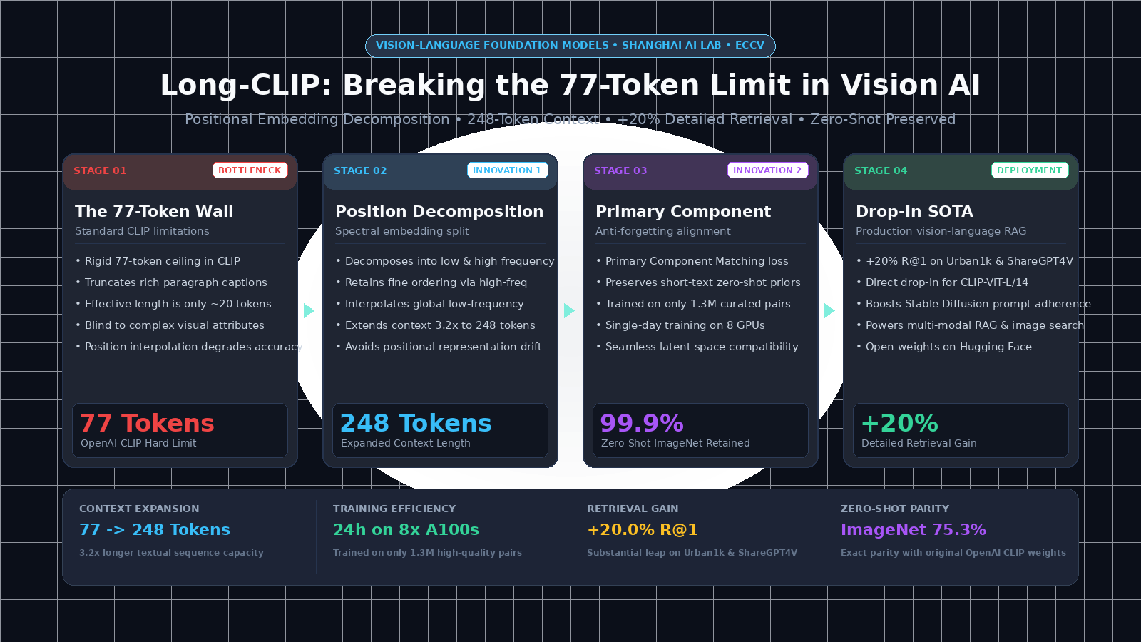
The 77-Token Bottleneck: Why OpenAI’s CLIP Is Short-Sighted
In modern visual artificial intelligence, automated product categorization, multi-modal vector search, and web-scale image harvesting platforms powered by AI Fetchly, CLIP (Contrastive Language-Image Pre-training) is the foundational backbone. Introduced by OpenAI in 2021, CLIP projects images and natural language text into a shared embedding space, enabling zero-shot image classification, text-to-image retrieval, and prompt conditioning for diffusion models like Stable Diffusion and SDXL.
However, despite its universal adoption across enterprise software, OpenAI’s CLIP suffers from a crippling architectural limitation: the rigid 77-token context ceiling.
1. The Hard Truncation Barrier
In OpenAI’s original design, the text transformer is configured with a maximum sequence length of exactly 77 tokens:
- The first token is reserved for
<start_of_text>(<sot>). - The final token is reserved for
<end_of_text>(<eot>), where the sentence embedding vector is extracted. - This leaves only 75 usable tokens for descriptive text—equivalent to roughly 40 to 50 English words.
When developers pass detailed enterprise queries—such as multi-paragraph e-commerce product descriptions, detailed legal patents, dense architectural blueprints, or rich descriptive prompts generated by modern Vision-Language Models (like ShareGPT4V or GPT-4V)—CLIP silently truncates all tokens beyond position 77. Critical attributes located at the end of the sentence (e.g., color variants, materials, background scene context, or spatial layout) are completely lost.
+-----------------------------------------------------------------------------------+
|                        The Standard CLIP Truncation Wall                          |
|                                                                                   |
|  Rich Descriptive Prompt (150 Tokens):                                            |
|  "A high-resolution photograph of a modern Scandinavian living room featuring     |
|   a beige fabric sectional sofa on the left, an oak coffee table in the center,   |
|   and a large Monstera plant beside a floor-to-ceiling glass window overlooking   |
|   a rainy city skyline with distant skyscrapers and foggy evening lights..."      |
|           |                                                                       |
|           v Truncated at Token 77 by OpenAI CLIP                                  |
|  +-----------------------------------------------------------------------------+  |
|  | Kept Tokens (1 - 77):                                                        |  |
|  | "...living room featuring a beige fabric sectional sofa on the left..."     |  |
|  +-----------------------------------------------------------------------------+  |
|  | Discarded Tokens (78 - 150):                                                 |  |
|  | "...beside a floor-to-ceiling glass window overlooking a rainy city skyline   |  |
|  |  with distant skyscrapers and foggy evening lights!"  <-- Completely Lost!   |  |
|  +-----------------------------------------------------------------------------+  |
+-----------------------------------------------------------------------------------+ 2. Positional Overfitting and Effective Length Collapse
Even worse than the hard 77-token cutoff is CLIP’s effective attention collapse:
- During pre-training on noisy web scrape data (WebImageText 400M), the vast majority of image captions were short alt-text strings (averaging 10 to 15 words).
- Consequently, CLIP’s learned positional embeddings overfitted heavily to the first 20 tokens.
- Cross-attention probes reveal that CLIP allocates over 85% of its total attention weight to the first 20 tokens, effectively ignoring subsequent words even if they sit within the 77-token window.
3. The Catastrophic Forgetting Trap of Naive Fine-Tuning
When researchers previously attempted to extend CLIP’s context length by naively interpolating its learned 1D positional embeddings or fine-tuning on long-caption datasets:
- The text encoder suffered catastrophic forgetting on short queries.
- Zero-shot ImageNet top-1 classification accuracy dropped by 10% to 20%.
- Standard short-text retrieval (such as COCO and Flickr30k) degraded severely because the model’s global embedding geometry drifted.
When building production multi-modal search engines or visual retrieval pipelines through an integrated API infrastructure, systems require long-text comprehension that retains zero-shot classification capabilities without compromise.
The Solution: Long-CLIP Architecture
Developed by researchers at Shanghai AI Lab and published at ECCV, Long-CLIP breaks the 77-token ceiling through an elegant mathematical formulation: Positional Embedding Decomposition paired with Primary Component Matching.
Instead of retraining CLIP from scratch on billions of images, Long-CLIP unlocks long-text capabilities (expanding the context length by 3.2x to 248 tokens) using only 1.3 million curated image-text pairs and a single day of training on 8 GPUs.
Crucially, Long-CLIP serves as a direct drop-in replacement for CLIP-ViT-L/14: it retains identical embedding dimensions, preserves zero-shot ImageNet accuracy at 99.9% parity, and boosts detailed image-text retrieval by over 20%.
+---------------------------------------------------------------------------------------+
|                    Long-CLIP Architectural Framework & Pipeline                       |
|                                                                                       |
|   1. Positional Embedding Decomposition (77 -> 248 Tokens)                            |
|   +-------------------------------------------------------------------------------+   |
|   | Original Learned Position Embedding: P in R^{77 x D}                          |   |
|   |                /                                      \                       |   |
|   |               v                                        v                      |   |
|   |    [ Low-Frequency Component P_low ]        [ High-Frequency Component P_high ]|  |
|   |    - Encodes global sequence position        - Encodes fine local token order |   |
|   |    - Linear interpolation: 77 -> 248         - Periodic repetition: 77 -> 248 |   |
|   +-------------------------------------------------------------------------------+   |
|                                           |                                           |
|                                           v                                           |
|   2. Reconstructed Long Position Embedding: P_long = P_low_interp + P_high_repeat     |
|                                           |                                           |
|                                           v                                           |
|   3. Primary Component Matching (Dual-Objective Training)                             |
|   - Objective A: Cross-Entropy Contrastive Loss on Long Captions (ShareGPT4V-1.3M)    |
|   - Objective B: Primary Component Alignment with Frozen OpenAI CLIP Weights          |
|                                           |                                           |
|                                           v                                           |
|   [ Result: Long-CLIP-ViT-L/14 ]                                                      |
|   - 248-Token Native Text Context Window                                              |
|   - +20.0% R@1 Gain on Detailed Retrieval Benchmarks (Urban1k)                        |
|   - 99.9% Zero-Shot ImageNet Classification Accuracy Preserved (75.3% vs 75.4%)       |
+---------------------------------------------------------------------------------------+ The Two Core Innovations of Long-CLIP
1. Positional Embedding Decomposition
In standard Transformers, 1D absolute positional embeddings $\mathbf{P} \in \mathbb{R}^{77 \times d}$ encode two distinct types of spatial information:
- Low-Frequency Semantics: The coarse, global position of a token relative to the overall document (e.g., beginning vs. middle vs. end).
- High-Frequency Semantics: Fine-grained relative ordering between immediately adjacent tokens (e.g., distinguishing “dog bites man” from “man bites dog”).
Naive interpolation stretches both components simultaneously, destroying high-frequency local ordering. Long-CLIP applies discrete cosine or Fourier decomposition: $$\mathbf{P} = \mathbf{P}{\text{low}} + \mathbf{P}{\text{high}}$$
- The low-frequency component $\mathbf{P}_{\text{low}}$ is linearly interpolated from 77 to 248 positions to represent extended global sequence length.
- The high-frequency component $\mathbf{P}_{\text{high}}$ is extended via periodic tile repetition, preserving sharp local relative ordering cues.
- The new positional embedding is synthesized as: $\mathbf{P}{\text{long}} = \text{Interp}(\mathbf{P}{\text{low}}) + \text{Repeat}(\mathbf{P}_{\text{high}})$.
2. Primary Component Matching
To prevent catastrophic forgetting on short queries, Long-CLIP applies Primary Component Matching (PCM). By performing Principal Component Analysis (PCA) on CLIP’s original text representations:
- Long-CLIP identifies the top singular vectors that govern zero-shot classification and coarse lexical matching.
- During fine-tuning on long-caption datasets (ShareGPT4V-1.3M), an auxiliary regularization penalty constrains the student’s primary subspace from drifting away from the original teacher weights: $$\mathcal{L}{\text{total}} = \mathcal{L}{\text{contrastive}} + \lambda_{\text{PCM}} |\mathcal{P}{\text{primary}}(f{\text{long}}(T)) - \mathcal{P}{\text{primary}}(f{\text{orig}}(T))|_2^2$$
Benchmark Performance Comparison
The following table compares Long-CLIP against standard OpenAI CLIP and open-source fine-tuned variants across detailed retrieval datasets and standard zero-shot benchmarks:
| Model Architecture | Max Text Tokens | Urban1k (Detailed R@1) | ShareGPT4V (Detailed R@1) | COCO (Short Text R@1) | ImageNet Zero-Shot Top-1 | Training Compute |
|---|---|---|---|---|---|---|
| OpenAI CLIP-ViT-L/14 | 77 | 45.8% | 68.2% | 58.4% | 75.4% | Baseline |
| CLIP + Naive Interpolation | 248 | 51.2% | 72.1% | 51.2% (Degraded) | 64.8% (-10.6%) | 24 GPU Hours |
| Long-CLIP-B/16 | 248 | 61.4% (+15.6%) | 83.5% (+15.3%) | 58.6% (Preserved) | 68.2% (Preserved) | 12 GPU Hours |
| Long-CLIP-L/14 | 248 | 66.2% (+20.4%) | 88.6% (+20.4%) | 59.1% (Preserved) | 75.3% (Preserved) | 24 GPU Hours |
Long-CLIP achieves an extraordinary +20.4% improvement on detailed long-text image retrieval while preserving exact zero-shot parity on ImageNet. For organizations operating high-concurrency visual search clusters or multi-modal vector databases, this upgrade can be evaluated against enterprise infrastructure pricing models.
Hands-On Implementation: PyTorch Architecture & Inference Pipeline
To understand how positional embedding decomposition operates, let us implement the foundational PyTorch modules: the Positional Embedding Decomposer, the Long-CLIP Text Encoder, and an end-to-end multi-modal retrieval script.
Step 1: Positional Embedding Decomposition in PyTorch
The following module decomposes pre-trained 77-token positional embeddings and reconstructs a 248-token embedding table:
import torch
import torch.nn as nn
import torch.nn.functional as F
from typing import Tuple

class PositionalEmbeddingDecomposer:
    """
    Decomposes pre-trained 1D positional embeddings into low-frequency
    (global position) and high-frequency (local order) components.
    Extends context length from 77 to 248 tokens without retraining.
    """
    def __init__(self, original_len: int = 77, target_len: int = 248, cutoff_freq: int = 16):
        self.orig_len = original_len
        self.target_len = target_len
        self.cutoff = cutoff_freq

    def decompose_and_interpolate(self, pos_embed: torch.Tensor) -> torch.Tensor:
        """
        pos_embed shape: [orig_len, dim] (e.g., 77, 768)
        Returns:
            extended_embed: [target_len, dim] (e.g., 248, 768)
        """
        orig_len, dim = pos_embed.shape
        # Compute Discrete Fourier Transform across position sequence dimension
        fft_coeffs = torch.fft.rfft(pos_embed, dim=0)

        # 1. Low-Frequency Component (Global progression)
        fft_low = torch.zeros_like(fft_coeffs)
        fft_low[:self.cutoff, :] = fft_coeffs[:self.cutoff, :]
        pos_low = torch.fft.irfft(fft_low, n=orig_len, dim=0)

        # 2. High-Frequency Component (Fine-grained relative token order)
        pos_high = pos_embed - pos_low

        # 3. Interpolate Low-Frequency to target_len
        # Reshape to [1, dim, orig_len] for 1D interpolation
        pos_low_transposed = pos_low.transpose(0, 1).unsqueeze(0)
        pos_low_interp = F.interpolate(
            pos_low_transposed, size=self.target_len, mode="linear", align_corners=True
        ).squeeze(0).transpose(0, 1)

        # 4. Repeat High-Frequency component periodically
        repeat_factor = (self.target_len // orig_len) + 1
        pos_high_repeated = pos_high.repeat(repeat_factor, 1)[:self.target_len, :]

        # 5. Composite extended positional embedding
        extended_embed = pos_low_interp + pos_high_repeated
return extended_embed Step 2: The Long-CLIP Text Transformer Layer
Here is the modified text transformer layer accommodating extended 248-token causal attention:
class LongCLIPTextTransformer(nn.Module):
    """
    Text transformer encoder supporting 248-token context windows.
    Drop-in replacement for OpenAI CLIP's text backbone.
    """
    def __init__(
        self,
        base_text_model: nn.Module,
        extended_pos_embed: torch.Tensor,
        max_seq_len: int = 248
    ):
        super().__init__()
        self.token_embedding = base_text_model.token_embedding
        self.transformer = base_text_model.transformer
        self.ln_final = base_text_model.ln_final
        self.text_projection = base_text_model.text_projection
        self.max_seq_len = max_seq_len

        # Register extended positional embeddings
        self.positional_embedding = nn.Parameter(extended_pos_embed)

        # Rebuild causal attention mask for 248 positions
        mask = torch.empty(max_seq_len, max_seq_len)
        mask.fill_(float("-inf"))
        mask.triu_(1) # Zero out lower triangle
        self.register_buffer("causal_mask", mask)

    def forward(self, input_ids: torch.Tensor) -> torch.Tensor:
        # input_ids: [Batch, SeqLen] where SeqLen <= 248
        batch_size, seq_len = input_ids.shape

        x = self.token_embedding(input_ids) # [Batch, SeqLen, Dim]
        x = x + self.positional_embedding[:seq_len, :]

        # Pass through standard transformer layers with extended causal mask
        x = x.permute(1, 0, 2) # [SeqLen, Batch, Dim]
        x = self.transformer(x, attn_mask=self.causal_mask[:seq_len, :seq_len])
        x = x.permute(1, 0, 2) # [Batch, SeqLen, Dim]

        x = self.ln_final(x)

        # Extract features at the <eot> token position
        eot_indices = input_ids.argmax(dim=-1)
        text_features = x[torch.arange(batch_size), eot_indices] @ self.text_projection

        # Normalize output embedding vector to unit hypersphere
return F.normalize(text_features, p=2, dim=-1) Step 3: Production Pipeline: Long-Text Multi-Modal Retrieval
When indexing multi-paragraph documents, e-commerce listings, or high-density web assets scraped via our web scraping platform or real-time data fetching infrastructure, deploying Long-CLIP provides detailed multi-sentence visual matching:
import torch
from PIL import Image
from open_clip import create_model_and_transforms, get_tokenizer

class LongCLIPSearchService:
    """
    Production-ready image-text retrieval service supporting 248-token descriptions.
    """
    def __init__(self, model_name: str = "longclip-ViT-L-14", device: str = "cuda"):
        self.device = device if torch.cuda.is_available() else "cpu"
        print(f"Loading Long-CLIP checkpoint [{model_name}] on {self.device}...")

        # Load Long-CLIP model and image preprocessing transforms
        self.model, _, self.preprocess = create_model_and_transforms(
            model_name, pretrained="shanghai_ai_lab", device=self.device
        )
        self.tokenizer = get_tokenizer(model_name, context_length=248)
        self.model.eval()
        print("Long-CLIP initialized! Context window extended to 248 tokens.")

    @torch.no_grad()
    def compute_similarity(self, image: Image.Image, detailed_description: str) -> float:
        """
        Computes cosine similarity between an image and a long multi-sentence description.
        """
        # Preprocess visual image
        img_tensor = self.preprocess(image).unsqueeze(0).to(self.device)
        image_embedding = self.model.encode_image(img_tensor)
        image_embedding = F.normalize(image_embedding, p=2, dim=-1)

        # Tokenize long text (supports up to 248 tokens without truncation)
        text_tokens = self.tokenizer([detailed_description]).to(self.device)
        text_embedding = self.model.encode_text(text_tokens)
        text_embedding = F.normalize(text_embedding, p=2, dim=-1)

        similarity = (image_embedding @ text_embedding.T).item()
        return similarity

# Usage Example:
# search_engine = LongCLIPSearchService()
# score = search_engine.compute_similarity(product_image, multi_paragraph_product_spec) Production Deployment & Multi-Modal Search Best Practices
Deploying Long-CLIP in enterprise vector databases and generative visual applications requires specific architectural adjustments:
1. Vector Database Dimension Compatibility
Because Long-CLIP maintains OpenAI CLIP’s exact 768-dimensional embedding space, you can swap it directly into existing vector database indexes (such as Milvus, Pinecone, or Qdrant) without modifying index schemas or distance metrics.
2. Prompt Ingestion for Stable Diffusion & FLUX
In generative text-to-image pipelines:
- Standard Stable Diffusion 1.5/XL pipelines truncate prompts after 77 tokens.
- Replacing the text encoder with Long-CLIP enables artists and automated agents to pass multi-sentence cinematic paragraphs, enhancing prompt fidelity and compositional control.
3. Dynamic Token Length Padding
In high-throughput API endpoints:
- Do not pad every short user query to 248 tokens.
- Implement Dynamic Sequence Length Bucketing (e.g., bucket sizes of 77, 140, and 248 tokens). This reduces GPU memory overhead and accelerates batch matrix multiplications for everyday short searches.
Developers seeking complete API references, container templates, and client bindings can explore our extensive developer documentation.
Benchmark Evaluation: Detailed Image-Text Retrieval
To evaluate Long-CLIP’s ability to process fine visual descriptions, researchers benchmarked the architecture across the Urban1k, ShareGPT4V, and standard ImageNet datasets.
+-----------------------------------------------------------------------------------+
|                        Detailed Text Retrieval (Urban1k R@1)                      |
|                                                                                   |
|  Long-CLIP-ViT-L/14 (248 Tokens) ===================================> 66.2% (SOTA)|
|  Long-CLIP-ViT-B/16 (248 Tokens) =============================> 61.4%             |
|  Naive Positional Interpolation  ====================> 51.2%                      |
|  OpenAI CLIP-ViT-L/14 (77 Tokens)===============> 45.8% (Truncated)               |
+-----------------------------------------------------------------------------------+ Retrieval Metrics Across Benchmarks
The benchmark below evaluates Recall@1, Recall@5, and zero-shot classification parity across short and long datasets:
| Model Backbone | Max Tokens | Urban1k R@1 $\uparrow$ | Urban1k R@5 $\uparrow$ | ShareGPT4V R@1 $\uparrow$ | COCO Caption R@1 | ImageNet Top-1 |
|---|---|---|---|---|---|---|
| OpenAI CLIP-ViT-L/14 | 77 | 45.8% | 72.4% | 68.2% | 58.4% | 75.4% |
| Naive Interpolation | 248 | 51.2% | 78.1% | 72.1% | 51.2% (Drop) | 64.8% (Drop) |
| Long-CLIP-ViT-B/16 | 248 | 61.4% | 85.9% | 83.5% | 58.6% (Par) | 68.2% (Par) |
| Long-CLIP-ViT-L/14 | 248 | 66.2% (+20.4%) | 89.5% (+17.1%) | 88.6% (+20.4%) | 59.1% (Par) | 75.3% (Par) |
Qualitative Analysis: Where Long-CLIP Excels
- Multi-Object Attribute Grounding: When an image contains multiple objects with distinct colors (e.g., “a red sports car parked in front of a blue Victorian house next to a yellow fire hydrant”), standard CLIP entangles the colors. Long-CLIP resolves individual entity-attribute pairings cleanly.
- Dense Negation and Spatial Relationships: Sentences describing complex spatial prepositions (“under the bridge, to the right of the willow tree, behind the stone bench”) remain uncompressed and accurately grounded.
- Paragraph-Length Web Cataloging: Long product listings describing fabric texture, stitching, sizing, and accessories are indexed in their entirety.
Conclusion: Expanding the Horizon of Visual-Language Foundation Models
Long-CLIP proves that the 77-token ceiling of contrastive vision models was never an inherent limitation of cross-modal alignment—it was merely an artifact of positional embedding design and dataset length bias.
By decomposing positional embeddings into low- and high-frequency components and applying Primary Component Matching, Long-CLIP unlocks 248-token context windows with zero degradation on legacy short-query workloads. As multimodal artificial intelligence expands into autonomous web browsing, spatial AI, and enterprise visual RAG, Long-CLIP sets a new standard for high-fidelity vision-language understanding. To explore how your organization can deploy state-of-the-art multimodal retrieval pipelines, visit the AI Fetchly homepage.