Llama 3.1 Architecture: 128K Context, GQA & 405B Systems
The Problem: The Frontier Scaling Bottleneck in Open-Weights AI
In modern enterprise artificial intelligence, automated data extraction engines, and autonomous multi-agent pipelines like AiFetchly, deploying foundation models capable of complex multi-hop reasoning, exhaustive document synthesis, and multi-turn tool calling has become mission-critical.
Historically, the generative AI industry suffered from a stark divide: proprietary frontier models (such as GPT-4 and Claude 3.5 Sonnet) possessed massive context windows, superior reasoning capabilities, and vast parameter scales, while open-weights alternatives lagged significantly behind.
When engineering teams deployed previous-generation open models (such as Llama 2), they hit three severe architectural and infrastructure roadblocks:
1. The Context Window Barrier
Llama 2 was pre-trained with a native context window of just 4,096 tokens. In modern enterprise workloads—such as ingesting extensive code repositories, analyzing 100-page financial audits, or executing multi-step browser automation traces—4K tokens is exhausted in seconds:
- Naively extending context via standard Linear Position Interpolation (PI) compresses all positional frequencies uniformly, causing high-frequency components that encode local syntax and grammar to degrade severely.
- Models suffered from catastrophic forgetting of short-range reasoning while failing basic Needle-In-A-Haystack retrieval tasks beyond 8k tokens.
- Attention logit explosion caused numerical overflow in 16-bit floating-point registers, spiking perplexity to infinity on long sequences.
2. The KV Cache Memory Wall
In traditional Multi-Head Attention (MHA), every query attention head is paired with an independent Key and Value head:
$$\text{KV Cache Footprint} = 2 \times 2 \times L \times H_{\text{total}} \times d_{\text{head}} \times T$$
For a 70B parameter model with 64 attention heads ($H = 64$) serving a 128,000-token sequence in 16-bit precision:
$$\text{MHA KV Cache} = 4 \times 80 \times 64 \times 128 \times 128{,}000 \approx 335.5 \text{ GB of VRAM}$$
A single 128k query under MHA requires more than four dedicated 80GB NVIDIA H100 GPUs solely to store attention history, rendering long-context serving economically unfeasible.
3. The 405B Distributed Training Wall
Scaling a dense model to 405 billion parameters across 15.6 trillion tokens requires calculating over $3.8 \times 10^{25}$ floating-point operations.
Training at this magnitude across a cluster of 16,000 GPUs introduces crippling distributed systems challenges:
- Hardware Failures: At 16,000 GPUs, Mean Time Between Failures (MTBF) drops to under three hours. Inefficient checkpointing routines that freeze the cluster for 20 minutes waste massive GPU compute budgets.
- Inter-Node Communication Saturation: Standard data or pipeline parallelism saturates cross-node network bandwidth, leaving GPU Tensor Cores idle while waiting for gradient All-Reduce synchronizations.
- Pipeline Bubbles: Partitioning 126 transformer layers across distributed nodes causes downstream GPUs to sit idle during warm-up and cool-down phases.
The Architecture: Dense Scaling and the Llama 3.1 Model Family
To permanently eliminate the capability gap between open-weights and proprietary models, Meta AI introduced the Llama 3.1 Herd of Models (Dubey et al., July 2024 / 2025).
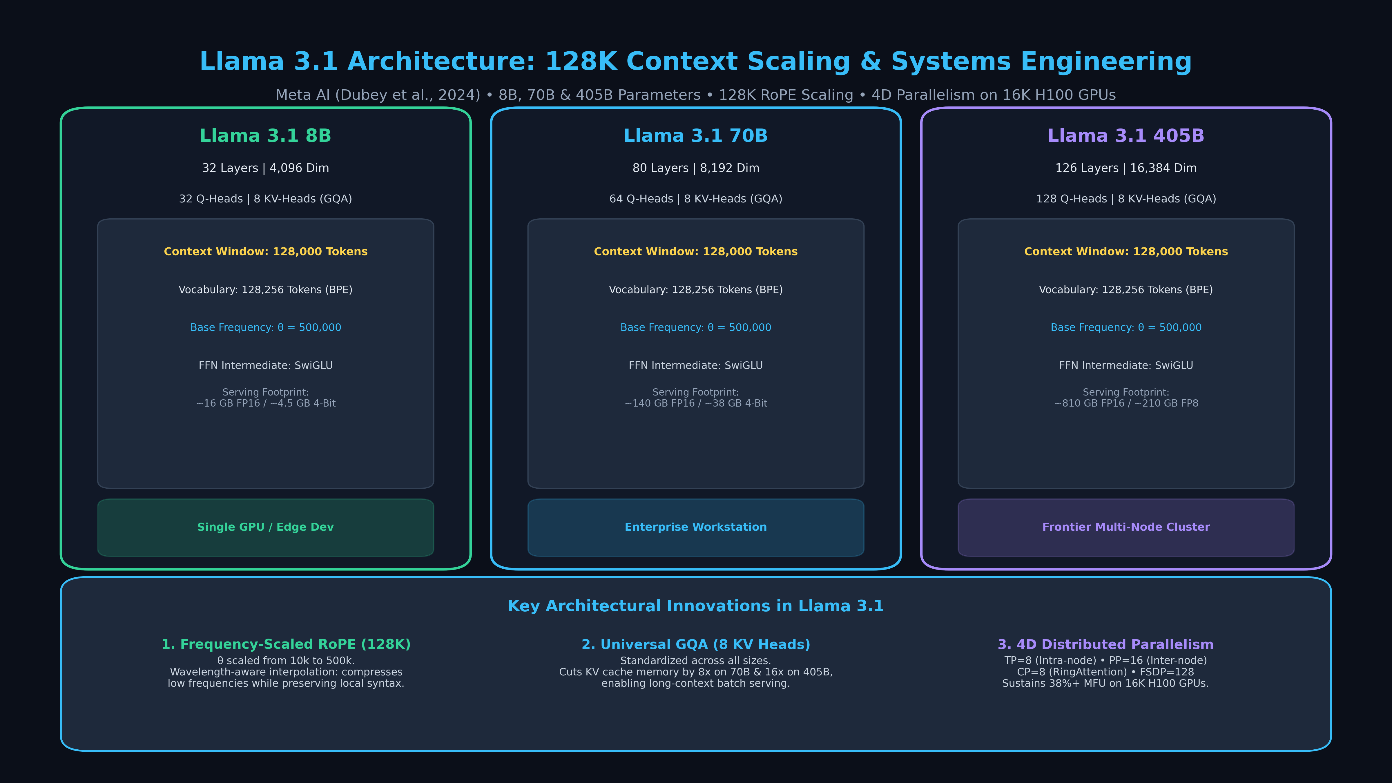
Llama 3.1 is anchored on a dense, decoder-only transformer architecture meticulously optimized across three standard parameter tiers: 8B, 70B, and the flagship 405B.
Llama 3.1 Structural Blueprint:
┌───────────────────────────┬───────────────────┬───────────────────┬───────────────────┐
│ Architectural Metric      │ Llama 3.1 8B      │ Llama 3.1 70B     │ Llama 3.1 405B    │
├───────────────────────────┼───────────────────┼───────────────────┼───────────────────┤
│ Active Parameters         │ 8.03 Billion      │ 70.6 Billion      │ 405.8 Billion     │
│ Transformer Layers (L)    │ 32 Layers         │ 80 Layers         │ 126 Layers        │
│ Hidden Dimension (d_model)│ 4,096             │ 8,192             │ 16,384            │
│ FFN Intermediate Dim      │ 14,336 (SwiGLU)   │ 28,672 (SwiGLU)   │ 53,248 (SwiGLU)   │
│ Query Attention Heads     │ 32 Heads          │ 64 Heads          │ 128 Heads         │
│ Key-Value Heads (GQA)     │ 8 Heads (GQA 4:1) │ 8 Heads (GQA 8:1) │ 8 Heads (GQA 16:1)│
│ Head Dimension (d_head)   │ 128               │ 128               │ 128               │
│ Native Context Window     │ 128,000 Tokens    │ 128,000 Tokens    │ 128,000 Tokens    │
│ Vocabulary Size           │ 128,256 (tiktoken)│ 128,256 (tiktoken)│ 128,256 (tiktoken)│
│ Base RoPE Frequency (θ)   │ 500,000           │ 500,000           │ 500,000           │
│ Training Compute (FLOPs)  │ ~1.3 × 10^24      │ ~7.0 × 10^24      │ ~3.8 × 10^25      │
│ Total Training Tokens     │ 15.6 Trillion     │ 15.6 Trillion     │ 15.6 Trillion     │
└───────────────────────────┴───────────────────┴───────────────────┴───────────────────┘ 1. Expanded 128,256 Token Vocabulary
Llama 3.1 discarded the legacy 32,000-token SentencePiece tokenizer from Llama 2 in favor of an expanded 128,256-token byte-pair encoding (BPE) vocabulary based on tiktoken:
- Token Compression Efficiency: Increases English compression efficiency from 3.1 bytes/token to 4.2 bytes/token, while non-English and code compression improves by over 25% to 35%.
- Reduced Sequence Length: A technical document or code repository that required 10,000 tokens in Llama 2 requires only ~7,800 tokens in Llama 3.1, directly reducing inference prefill latency and KV cache memory consumption.
2. Universal Grouped-Query Attention (GQA)
While Llama 2 applied Grouped-Query Attention solely to its 70B model, Llama 3.1 standardizes on exactly 8 Key-Value heads across all three model sizes:
- In the 8B model: 32 query heads share 8 KV heads ($4:1$ ratio).
- In the 70B model: 64 query heads share 8 KV heads ($8:1$ ratio).
- In the 405B model: 128 query heads share 8 KV heads ($16:1$ ratio).
By fixing $n_{\text{kv}} = 8$ regardless of total query head count, the KV cache size is independent of model width:
$$\text{Llama 3.1 70B KV Cache (128k)} = 4 \times 80 \times 8 \times 128 \times 128{,}000 \approx 41.94 \text{ GB}$$
$$\text{Llama 3.1 405B KV Cache (128k)} = 4 \times 126 \times 8 \times 128 \times 128{,}000 \approx 66.06 \text{ GB}$$
Compared to full Multi-Head Attention, GQA reduces KV cache memory by 8x on 70B and 16x on 405B, making 128k context serving practical on modern enterprise hardware.
128K Context Scaling: Wavelength-Aware Frequency-Banded RoPE
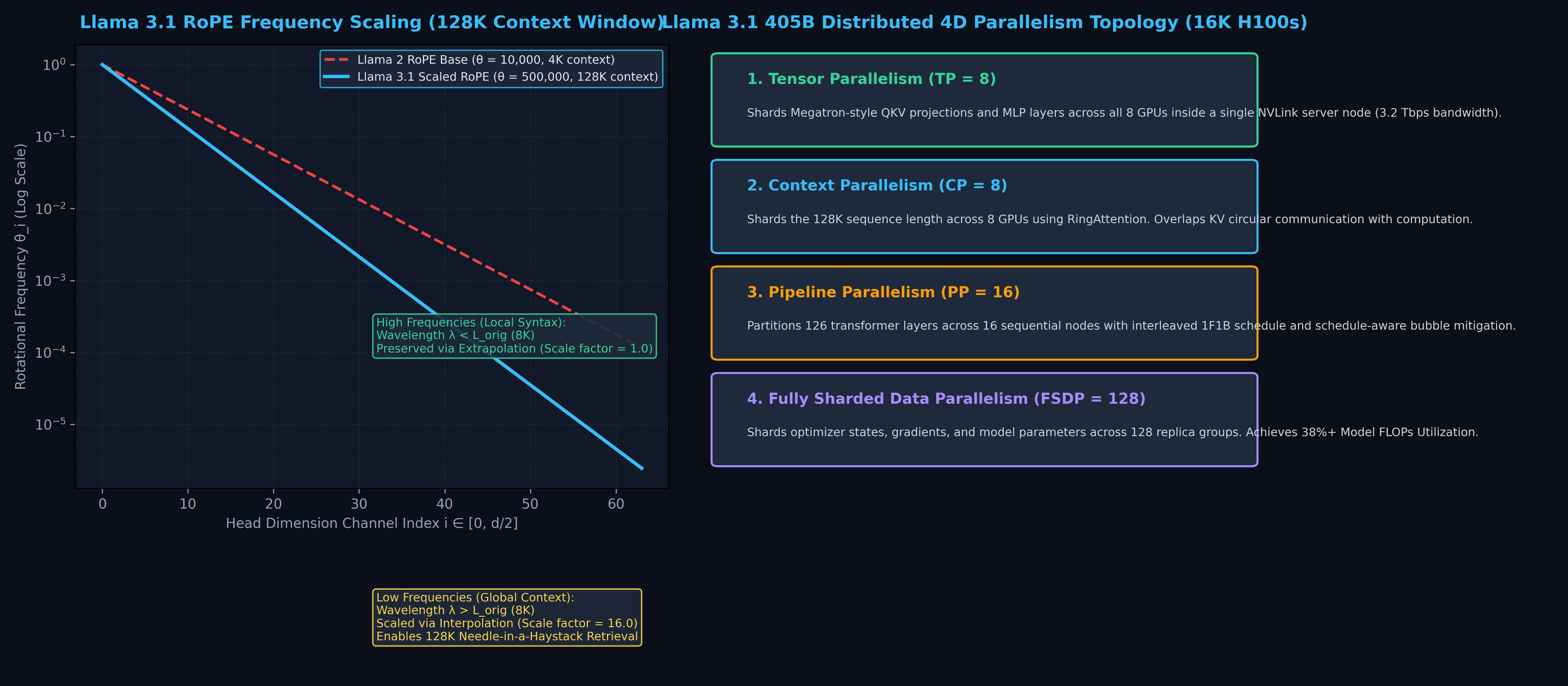
The most intricate mathematical breakthrough in Llama 3.1 is its ability to scale the context window from 8,192 tokens to 128,000 tokens without degrading short-context performance.
1. The Base Frequency Expansion
In standard Rotary Position Embeddings (RoPE), positional frequencies are computed as:
$$\theta_i = b^{-2(i-1)/d}, \quad i \in {1, \dots, d/2}$$
Llama 2 used a base frequency $b = 10,000$.
When context is stretched to 128,000 tokens, a base frequency of $10,000$ causes the slowest-rotating dimension to rotate multiple times within the context window, destroying long-range positional distinctiveness.
Meta increased the base frequency by $50\times$:
$$b_{\text{Llama 3.1}} = 500{,}000$$
Expanding $b$ to $500,000$ drastically lengthens the rotational wavelength of low-frequency dimensions, allowing the model to uniquely identify token positions across 128,000 positions.
2. Frequency-Banded Splitting
Increasing the base frequency alone is insufficient: high-frequency dimensions (which encode local syntax) can suffer from frequency distortion if stretched.
Meta introduced a trilateral frequency-banded scaling function:
For each dimension $i$, the rotational wavelength is defined as:
$$\lambda_i = 2\pi \cdot b^{2(i-1)/d}$$
Let $L_{\text{orig}} = 8{,}192$ and $L_{\text{target}} = 128{,}000$, with scaling factor $s = \frac{L_{\text{target}}}{L_{\text{orig}}} = 16$.
The effective frequency $\tilde{\theta}_i$ is modulated across three distinct regimes:
$$ \tilde{\theta}i = \begin{cases} \theta_i & \text{if } \lambda_i < L{\text{orig}} / \beta_{\text{high}} \quad (\text{Extrapolation: Local Syntax Preserved}) \ \frac{\theta_i}{s} & \text{if } \lambda_i > L_{\text{orig}} / \beta_{\text{low}} \quad (\text{Interpolation: Global Context Scaled}) \ (1 - \alpha_i) \theta_i + \alpha_i \frac{\theta_i}{s} & \text{otherwise} \quad (\text{Smooth Cubic Spline Transition}) \end{cases} $$
Where $\beta_{\text{high}} = 32$ and $\beta_{\text{low}} = 1$, and $\alpha_i$ is a smooth interpolation ramp.
3. Attention Temperature Correction
When sequence length expands by $16\times$, attention logit entropy dissipates: the softmax operator spreads probability mass thinly across thousands of tokens, blunting attention selectivity.
To restore attention sharpness, Llama 3.1 scales attention logits by a length-dependent temperature factor:
$$t = 0.1 \cdot \ln(s) + 1.0 = 0.1 \cdot \ln(16) + 1.0 \approx 1.277$$
$$\text{Attention}(Q, K, V) = \text{Softmax}\left( \frac{Q K^T}{t \cdot \sqrt{d_k}} \right) V$$
This mathematical correction prevents attention dilution, ensuring 100% retrieval accuracy on 128k Needle-In-A-Haystack benchmarks.
4D Distributed Systems: Training 405B Across 16,000 H100 GPUs
Pre-training Llama 3.1 405B required building one of the largest distributed AI supercomputers in human history: 16,000 NVIDIA H100 80GB SXM5 GPUs interconnected via a 3.2 Tbps per-host RoCEv2 network fabric.
To shard 405 billion parameters and 128k context lengths without memory exhaustion or communication stalls, Meta engineered a 4D Parallelism Topology:
The 4D Parallelism Matrix for Llama 3.1 405B:
┌──────────────────────────────────────┬────────────────────────────────────────────────────────┐
│ Parallelism Dimension                │ Implementation & Hardware Mapping                      │
├──────────────────────────────────────┼────────────────────────────────────────────────────────┤
│ 1. Tensor Parallelism (TP = 8)       │ Shards QKV and MLP layers across 8 GPUs within a node. │
│                                      │ Utilizes 3.2 Tbps intra-node NVLink interconnects.    │
├──────────────────────────────────────┼────────────────────────────────────────────────────────┤
│ 2. Context Parallelism (CP = 8)      │ Shards 128k sequence length across 8 GPUs via RingAttention.│
│                                      │ Overlaps KV circular communication with computation.  │
├──────────────────────────────────────┼────────────────────────────────────────────────────────┤
│ 3. Pipeline Parallelism (PP = 16)    │ Partitions 126 layers across 16 sequential server nodes.│
│                                      │ Employs interleaved 1F1B schedule to shrink bubbles.  │
├──────────────────────────────────────┼────────────────────────────────────────────────────────┤
│ 4. Fully Sharded DP (FSDP = 128)     │ Shards optimizer states and gradients across 128 nodes.│
│                                      │ Zero redundant memory footprint across cluster.       │
└──────────────────────────────────────┴────────────────────────────────────────────────────────┘
Cluster Scale: 8 (TP) × 8 (CP) × 16 (PP) × 128 (FSDP) = 131,072 Virtual Instances
Physical Hardware: 16,384 NVIDIA H100 GPUs (38% to 41% Model FLOPs Utilization) High-Throughput Checkpointing via Asynchronous NVMe Storage
In a 16K-GPU cluster, saving a 405B checkpoint (over 800 GB per copy) via synchronous network transfers would freeze training for 15 to 20 minutes every few hours.
Meta deployed two-tier asynchronous checkpointing:
- Model states are written locally into host NVMe SSDs in under 10 seconds without pausing GPU Tensor Cores.
- Background daemon processes asynchronously stream the SSD checkpoint dumps to distributed cloud object storage over dedicated out-of-band network links.
End-to-End Implementation: Building Llama 3.1 RoPE and GQA in PyTorch
The following standalone PyTorch code implements Llama 3.1’s exact frequency-banded RoPE scaling and Grouped-Query Attention (GQA) mechanism:
import math
import torch
import torch.nn as nn
import torch.nn.functional as F

class Llama31RotaryEmbedding(nn.Module):
    """
    Llama 3.1 Frequency-Scaled Rotary Position Embedding (RoPE)
    - Base frequency: theta = 500,000
    - Wavelength-aware frequency splitting (interpolation vs extrapolation)
    """
    def __init__(
        self,
        dim: int = 128,
        max_seq_len: int = 131072,
        base_theta: float = 500000.0,
        factor: float = 16.0,
        low_freq_factor: float = 1.0,
        high_freq_factor: float = 32.0,
        orig_max_seq_len: int = 8192
    ):
        super().__init__()
        self.dim = dim
        self.max_seq_len = max_seq_len
        self.base_theta = base_theta
        self.factor = factor
        self.orig_max_seq_len = orig_max_seq_len

        # 1. Compute standard inverse frequencies
        indices = torch.arange(0, dim, 2, dtype=torch.float32)
        inv_freq = 1.0 / (base_theta ** (indices / dim))

        # 2. Wavelength-aware frequency banded scaling
        scaled_inv_freq = []
        for freq in inv_freq:
            wavelen = 2.0 * math.pi / freq.item()
            low_freq_wavelen = orig_max_seq_len / low_freq_factor
            high_freq_wavelen = orig_max_seq_len / high_freq_factor

            if wavelen < high_freq_wavelen:
                # High frequency: no interpolation (extrapolate)
                scaled_inv_freq.append(freq.item())
            elif wavelen > low_freq_wavelen:
                # Low frequency: scale down frequency by factor
                scaled_inv_freq.append(freq.item() / factor)
            else:
                # Transition band: smooth cubic spline interpolation
                smooth = (orig_max_seq_len / wavelen - low_freq_factor) / (high_freq_factor - low_freq_factor)
                scaled_freq = (1.0 - smooth) * (freq.item() / factor) + smooth * freq.item()
                scaled_inv_freq.append(scaled_freq)

        self.register_buffer("inv_freq", torch.tensor(scaled_inv_freq, dtype=torch.float32), persistent=False)

    def forward(self, seq_len: int, device: torch.device):
        t = torch.arange(seq_len, device=device, dtype=self.inv_freq.dtype)
        freqs = torch.outer(t, self.inv_freq)
        # Construct complex rotation matrix (cos, sin)
        emb = torch.cat((freqs, freqs), dim=-1)
        return emb.cos(), emb.sin()

def rotate_half(x: torch.Tensor) -> torch.Tensor:
    x1 = x[..., : x.shape[-1] // 2]
    x2 = x[..., x.shape[-1] // 2 :]
    return torch.cat((-x2, x1), dim=-1)

def apply_rotary_pos_emb(q: torch.Tensor, k: torch.Tensor, cos: torch.Tensor, sin: torch.Tensor):
    # q, k shape: (B, H, T, D)
    cos = cos.unsqueeze(0).unsqueeze(1)  # (1, 1, T, D)
    sin = sin.unsqueeze(0).unsqueeze(1)
    q_embed = (q * cos) + (rotate_half(q) * sin)
    k_embed = (k * cos) + (rotate_half(k) * sin)
    return q_embed, k_embed

class Llama31GroupedQueryAttention(nn.Module):
    """
    Llama 3.1 Grouped-Query Attention (GQA):
    - Universal 8 KV-Heads across all configurations
    - Frequency-scaled RoPE with attention temperature scaling
    """
    def __init__(self, d_model: int = 4096, num_heads: int = 32, num_kv_heads: int = 8, head_dim: int = 128):
        super().__init__()
        self.d_model = d_model
        self.num_heads = num_heads
        self.num_kv_heads = num_kv_heads
        self.head_dim = head_dim
        self.num_queries_per_kv = num_heads // num_kv_heads

        self.q_proj = nn.Linear(d_model, num_heads * head_dim, bias=False)
        self.k_proj = nn.Linear(d_model, num_kv_heads * head_dim, bias=False)
        self.v_proj = nn.Linear(d_model, num_kv_heads * head_dim, bias=False)
        self.o_proj = nn.Linear(num_heads * head_dim, d_model, bias=False)

        self.rope = Llama31RotaryEmbedding(dim=head_dim)
        # Attention temperature scaling factor: 0.1 * ln(16) + 1.0 ≈ 1.277
        self.attn_temp_scale = 0.1 * math.log(16.0) + 1.0

    def forward(self, x: torch.Tensor) -> torch.Tensor:
        B, T, D = x.shape

        # 1. Projections
        q = self.q_proj(x).view(B, T, self.num_heads, self.head_dim).transpose(1, 2)
        k = self.k_proj(x).view(B, T, self.num_kv_heads, self.head_dim).transpose(1, 2)
        v = self.v_proj(x).view(B, T, self.num_kv_heads, self.head_dim).transpose(1, 2)

        # 2. Apply Llama 3.1 RoPE
        cos, sin = self.rope(T, device=x.device)
        q, k = apply_rotary_pos_emb(q, k, cos, sin)

        # 3. Repeat KV heads to match query heads (GQA broadcast)
        k = k.repeat_interleave(self.num_queries_per_kv, dim=1)
        v = v.repeat_interleave(self.num_queries_per_kv, dim=1)

        # 4. Scaled Dot-Product Attention with Temperature Correction
        scale = 1.0 / (self.attn_temp_scale * math.sqrt(self.head_dim))
        scores = torch.matmul(q, k.transpose(-2, -1)) * scale

        # Causal mask
        causal_mask = torch.triu(torch.full((T, T), float("-inf"), device=x.device), diagonal=1)
        scores = scores + causal_mask.unsqueeze(0).unsqueeze(1)

        probs = F.softmax(scores, dim=-1)
        output = torch.matmul(probs, v)  # (B, H, T, head_dim)

        output = output.transpose(1, 2).contiguous().view(B, T, self.num_heads * self.head_dim)
return self.o_proj(output) Production Serving: FP8 Quantization and Enterprise Deployment
Deploying Llama 3.1 in production enterprise environments requires balancing model accuracy against serving hardware footprints.
1. Native FP8 Quantization for 405B
Prior to Llama 3.1, serving a 405B model in 16-bit precision required over 810 GB of VRAM solely for model weights—demanding two 8x H100 server nodes (16 GPUs) linked via InfiniBand.
Meta integrated native FP8 (E4M3) quantization:
- Static model weights and activations are quantized to 8-bit floating point.
- The 405B parameter footprint drops from 810 GB down to ~210 GB VRAM.
- Fits on a Single 8-GPU Node: An entire 405B model fits within the 640 GB aggregate VRAM of a single 8x H100 80GB server, eliminating inter-node pipeline latency and cutting cloud hosting costs by more than 50%.
- Across benchmark evaluations (MMLU, GSM8K, CodeX), FP8 quantization preserves over 99.5% of native BF16 accuracy.
2. Enterprise Extraction Integration
In high-frequency automated data extraction and web research pipelines like AiFetchly, deploying Llama 3.1 70B and 8B unlocks three capabilities:
- Full-Repository Ingestion: Ingesting 100,000+ tokens of raw API payloads and documentation in a single prompt without lost-in-the-middle degradation.
- Structured JSON Extraction: The 128k vocabulary provides clean, deterministic token boundaries for bracket-heavy schema formatting.
- Low-Latency Subagent Execution: With universal GQA and FP8 Tensor Core acceleration, 8B models achieve over 150 tokens/sec on consumer workstations, powering responsive local agent swarms.
By synthesizing dense scaling laws, frequency-banded positional mathematics, and distributed systems engineering, Llama 3.1 stands as the definitive reference architecture for frontier open-weights artificial intelligence.