liquid-foundation-modelslfmdynamical-systemsllm-architecturestate-space-modelstutorial

Liquid Foundation Models: Non-Transformer Architecture Guide

September 25, 2026

Liquid Foundation Models Architecture: Comparing Transformers, State Space Models, and LFM Adaptive Linear Operators

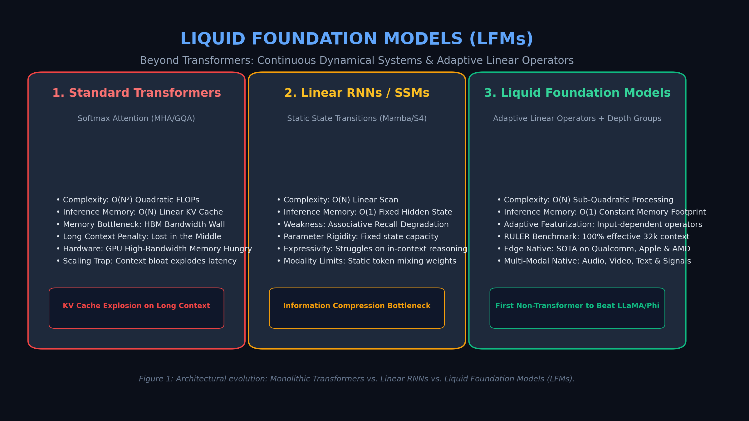
The Problem: The Inherent Constraints of the Transformer Architecture

For nearly a decade, the generative artificial intelligence industry has operated under a single computational paradigm: the Generative Pre-trained Transformer (GPT). From frontier multi-modal reasoning engines down to compact edge models and automated research assistants like AiFetchly, the Softmax Multi-Head Self-Attention mechanism has stood as the unchallenged default.

However, as production workloads demand extreme context windows (32k, 128k, and 1M+ tokens), edge device deployment (on phones, automotive chips, and IoT microcontrollers), and multi-modal continuous signal processing, the structural limitations of the Transformer have become an unsustainable engineering liability.

Deploying Transformers in modern high-throughput environments exposes three critical physical and mathematical bottlenecks:

1. The Quadratic Compute Wall: $O(N^2)$ Prefill FLOPs

Standard Multi-Head Attention computes dense pairwise dot-products across every token pair in an input sequence. For a sequence length $N$, the computational complexity scales quadratically:

$$\text{Attention FLOPs} = \mathcal{O}(N^2 \cdot d)$$

While GPU kernel optimizations like FlashAttention-2 and FlashAttention-3 minimize memory round-trips by tiling computations inside high-speed SRAM, they cannot alter the fundamental algorithmic complexity. When an autonomous agent ingests a 64,000-token enterprise document set, the attention layer computes over 4.29 billion pairwise interactions per attention head. On long sequences, prompt prefill computation saturates GPU Streaming Multiprocessors (SMs), driving Time-to-First-Token (TTFT) latency into multiple seconds.

2. The Linear KV Cache Explosion: The Memory Bandwidth Squeeze

During the autoregressive decoding phase—where the model generates tokens one by one—the Transformer must retain precomputed Key and Value projection tensors for all historical tokens in GPU High-Bandwidth Memory (HBM):

$$\text{KV Cache Memory (Bytes)} = 2 \times 2 \times L \times n_{\text{kv}} \times d_{\text{head}} \times N$$

For a 70B parameter model serving a 32k context, the KV cache alone consumes over 20 GB of VRAM per concurrent user request.

Because GPU memory capacity is strictly finite (e.g., 80 GB on an NVIDIA H100), serving systems face the Memory Bandwidth Wall:

During generation, modern GPU Tensor Cores sit idle for over 80% of clock cycles, starved of data while the memory controller attempts to stream gigabytes of cached keys and values across the memory bus just to compute one new token.
High concurrency collapses batch sizes, leading to massive cloud infrastructure expenditures and Out-of-Memory (OOM) crashes during traffic surges.

3. The Shortcomings of Prior Non-Transformer Systems

To break the quadratic barrier, researchers developed alternative sequence architectures, including State Space Models (SSMs) like Mamba-1/2, Linear Transformers, and Recurrent Neural Networks (RWKV-6). While these models achieve linear $O(N)$ training and constant $O(1)$ inference memory, they introduced new failure modes:

Associative Recall Degradation: Compressing historical context into a static, fixed-size hidden state causes linear models to fail on complex associative retrieval tasks (such as Multi-Query Associative Recall or needle-in-a-haystack lookups).
Static Token Mixing: Traditional SSMs rely on fixed parameter matrices ($A, B, C$) that do not adapt dynamically based on the input context, limiting in-context learning capabilities.
The Transformer Performance Gap: On rigorous academic benchmarks like MMLU, GSM8K, and HumanEval, pure SSMs consistently trailed transformer baselines at identical parameter scales.

The industry required an entirely new mathematical formulation: an architecture delivering the expressive reasoning power of transformers with the constant-memory speed of linear state-space models.

The Architecture: How Liquid Foundation Models Operate

To move beyond the limitations of Transformers, researchers at Liquid AI (pioneered by Hasani, Lechner, Rus, and colleagues at MIT CSAIL) introduced Liquid Foundation Models (LFMs).

Unlike architectures designed merely as heuristics over transformers, LFMs are built from first principles rooted in continuous-time dynamical systems, signal processing, and numerical linear algebra.

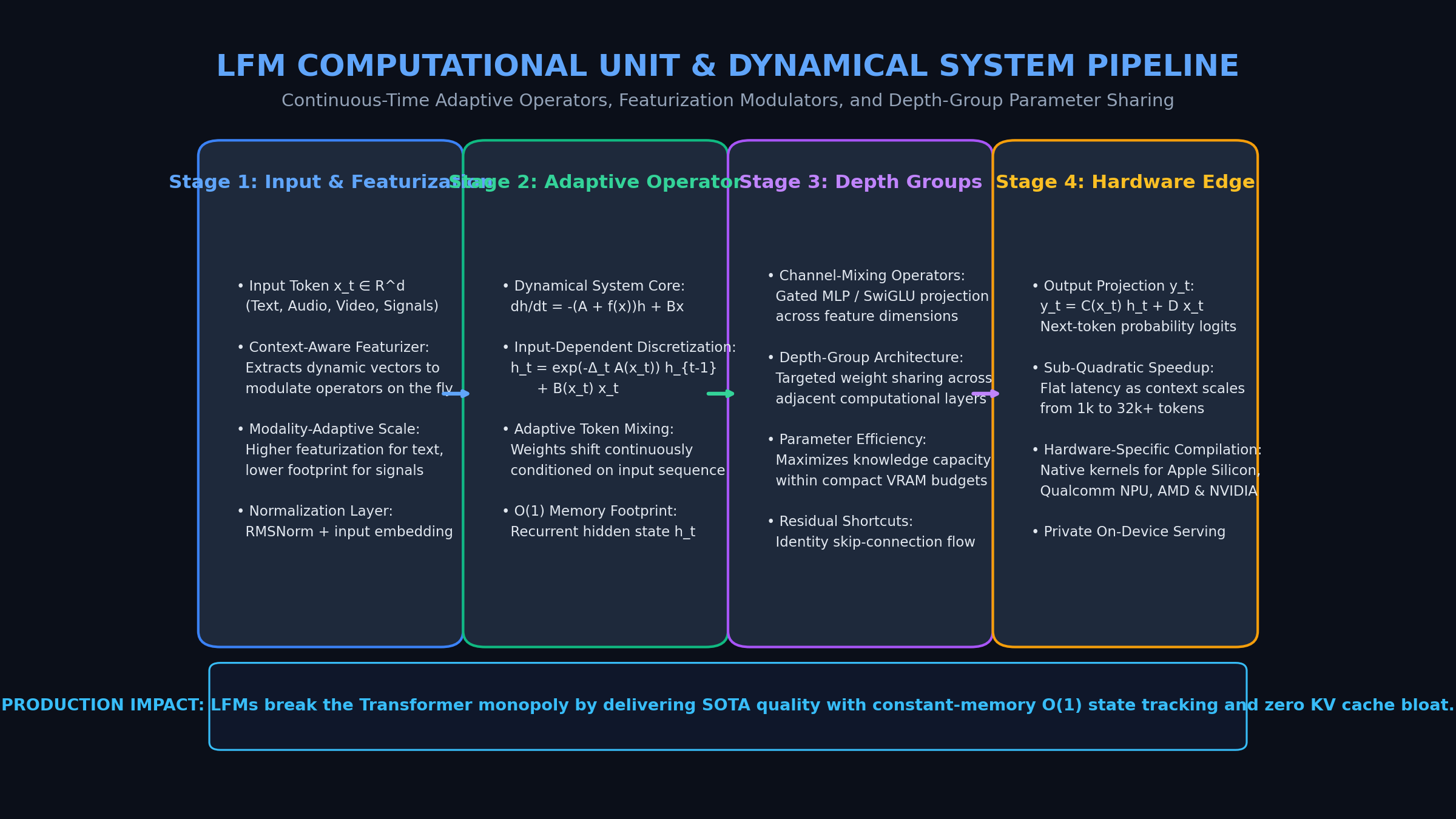
LFM Computational Unit and Dynamical System Pipeline: Featurization, Adaptive Operators, Depth Groups, and Edge Hardware

1. Continuous-Time Dynamical Systems as Computational Units

The intellectual foundation of LFMs stems from Liquid Neural Networks (LNNs)—neural models governed by nonlinear differential equations where the state dynamics evolve continuously over time:

$$\frac{d\mathbf{h}(t)}{dt} = -\left[ \mathbf{A} + f(\mathbf{x}(t)) \right] \mathbf{h}(t) + \mathbf{B} \mathbf{x}(t)$$

$$\mathbf{y}(t) = \mathbf{C} \mathbf{h}(t) + \mathbf{D} \mathbf{x}(t)$$

Where:

$\mathbf{h}(t) \in \mathbb{R}^d$ represents the hidden state vector.
$\mathbf{x}(t) \in \mathbb{R}^m$ is the incoming input signal at time $t$.
$\mathbf{A} \in \mathbb{R}^{d \times d}$ is a state decay matrix ensuring bounded stability.
$f(\mathbf{x}(t))$ is a learned, input-dependent nonlinear modulation function that dynamically adjusts the time-constant and transition speed of the state.

Because the system is continuous, the effective parameters of the network are “liquid”—they vary continuously as a function of incoming inputs rather than remaining static after training. When discretized for digital hardware using exact exponential integrators, the recurrent update becomes:

$$\mathbf{h}_t = \exp\left(-\Delta_t \left[\mathbf{A} + f(\mathbf{x}t)\right]\right) \mathbf{h}{t-1} + \mathbf{B}(\mathbf{x}_t) \mathbf{x}_t$$

2. Adaptive Linear Operators: Input-Dependent Token Mixing

At the core of language LFMs sits the Adaptive Linear Operator. In standard transformers, the token-mixing operator is the Softmax Attention matrix:

$$\mathbf{A}_{\text{attn}} = \text{Softmax}\left(\frac{\mathbf{Q} \mathbf{K}^T}{\sqrt{d}}\right)$$

In LFMs, token mixing is achieved through structured linear operators whose transformation properties are modulated directly by input features:

Featurization: The input sequence passes through a specialized featurizer module that extracts statistical and semantic features tailored to the data modality (text, audio, video, or time-series).
Dynamic Modulation: These extracted features dynamically parameterize the token-mixing operator, enabling the model to adjust its receptive field, decay rate, and attention focus on the fly.
Zero KV Cache Allocation: Unlike Transformers that store growing sequence histories in VRAM, the LFM maintains only the current compact hidden state $\mathbf{h}_t$. As sequence length scales from 1,000 to 32,000+ tokens, inference memory remains strictly constant $O(1)$.

To maximize knowledge capacity while keeping parameter counts lightweight for edge deployment, LFMs introduce Depth Groups:

Rather than assigning completely independent weight matrices to every single layer, the model organizes sequential layers into depth groups.
Within each depth group, core structured operators share underlying parameter representations while maintaining specialized input-dependent modulation heads.
This targeted weight sharing maximizes parameter utilization, allowing a 1.3B or 3.1B parameter LFM to achieve the factual knowledge capacity and benchmark accuracy of 7B+ parameter transformer models.

4. Empirical Performance: The First Non-Transformer to Beat LLaMA & Phi

In rigorous empirical evaluations using EleutherAI’s lm-evaluation-harness, Liquid Foundation Models demonstrated state-of-the-art results across compact scales:

The 1B Model Frontier

LFM-1B (1.3B parameters) achieves an MMLU score of 58.55 (5-shot), outperforming Meta’s Llama 3.2 1.2B (45.46), Microsoft’s Phi 1.5 1.4B (42.26), and RWKV-6 1.6B (26.02).
On GSM8K math reasoning, LFM-1B scores 55.34, outscoring Llama 3.2 1.2B (33.36) by over 20 percentage points.

The 3B Model Frontier

LFM-3B (3.1B parameters) achieves an MMLU score of 66.16 and GSM8K score of 70.28, rivaling Google’s Gemma 2 2.6B and outperforming Mistral-7B v0.3 on multiple reasoning evaluations.

Context Length Utilization (The RULER Benchmark)

While many commercial models advertise 128k context windows, their effective retrieval accuracy degrades sharply beyond 4k or 8k tokens. On the synthetic RULER benchmark (where effective retrieval requires a score $\ge 85.6$):

Llama 3.2 3B claims 128k context but drops to 74.1 at 32k (effective length: 4k).
LFM-3B achieves 89.5 at 32k, maintaining 100% effective long-context recall across its entire context window while using a fraction of the inference VRAM.

Architectural Comparison: Transformers vs. SSMs vs. Liquid Foundation Models

Dimension	Standard Transformer (LLaMA-3)	Linear State Space (Mamba-2)	Liquid Foundation Model (LFM)
Foundational Theory	Softmax Dot-Product Attention	Linear Time-Invariant SSMs	Continuous-Time Dynamical Systems
Prefill Computational Complexity	$O(N^2)$ Quadratic FLOPs	$O(N)$ Linear Scan	$O(N)$ Sub-Quadratic Structured Operator
Inference Memory Footprint	$O(N)$ Monotonically growing KV Cache	$O(1)$ Static Hidden State	$O(1)$ Constant-Memory State Tracking
Token Mixing Mechanism	Softmax pairwise attention matrix	Convolutional + Selective SSM	Adaptive Input-Dependent Linear Operators
Parameter Architecture	Independent parameters per layer	Independent parameters per layer	Depth Groups with Targeted Weight Sharing
Multi-Modal Adaptability	Discrete tokenization required	Primarily sequential/1D	Native (Audio, Video, Text, Time-Series)
Hardware Efficiency	Memory-bandwidth bound during decoding	High hardware utilization	Platform-native (NPU, Apple Silicon, AMD)

Implementation: Simulating an LFM Computational Unit in Python

To understand how adaptive linear operators and continuous-time dynamical systems function, let us build a reference simulation of an LFM computational unit in Python using NumPy and PyTorch.

This implementation demonstrates:

Context-Aware Featurizer: Extracting input-dependent modulation vectors.
Adaptive Continuous Discretization: Dynamically adjusting decay rates $\Delta_t$ and transition matrices based on input tokens.
Constant-Memory Recurrence: Generating sequential outputs with strictly $O(1)$ state memory.

import torch
import torch.nn as nn
import torch.nn.functional as F
from typing import Tuple, Optional

class LFMFeaturizer(nn.Module):
    """
    Featurization module responsible for modulating computation
    based on the input context.
    """
    def __init__(self, d_model: int, d_feat: int):
        super().__init__()
        self.proj = nn.Linear(d_model, d_feat, bias=False)
        self.norm = nn.RMSNorm(d_feat)

    def forward(self, x: torch.Tensor) -> torch.Tensor:
        # x: [batch_size, seq_len, d_model]
        return F.silu(self.norm(self.proj(x)))

class AdaptiveLinearOperator(nn.Module):
    """
    Core LFM token-mixing operator derived from continuous-time dynamical systems.
    dh/dt = -[A + f(x)] h + B x
    """
    def __init__(self, d_model: int, d_state: int, d_feat: int):
        super().__init__()
        self.d_model = d_model
        self.d_state = d_state

        # Base stability matrix log(A) ensuring decay >= 0
        self.log_A = nn.Parameter(torch.randn(d_state))

        # Projection for input driving operator B(x)
        self.proj_B = nn.Linear(d_model, d_state, bias=False)

        # Projection for output observation operator C(x)
        self.proj_C = nn.Linear(d_model, d_state, bias=False)

        # Adaptive step-size/decay modulation f(x)
        self.proj_delta = nn.Linear(d_feat, d_state)

        # Direct skip connection D
        self.D = nn.Parameter(torch.ones(d_model))

    def forward(self, x: torch.Tensor, feat: torch.Tensor) -> torch.Tensor:
        """
        Forward pass operating in parallel mode for training (O(N) associative scan).
        """
        batch_size, seq_len, _ = x.shape

        # 1. Compute input-dependent step sizes (Delta_t)
        # Softplus ensures positive decay rates for numerical stability
        delta = F.softplus(self.proj_delta(feat)) # [B, L, d_state]

        # 2. Compute dynamic decay A_bar = exp(-delta * exp(log_A))
        A = torch.exp(self.log_A) # [d_state]
        decay = torch.exp(-delta * A) # [B, L, d_state]

        # 3. Input injection B_bar = delta * B(x)
        B_x = self.proj_B(x) # [B, L, d_state]
        u = delta * B_x # [B, L, d_state]

        # 4. Sequential state update simulation (recurrent scan)
        h = torch.zeros(batch_size, self.d_state, device=x.device, dtype=x.dtype)
        h_states = []

        for t in range(seq_len):
            h = decay[:, t, :] * h + u[:, t, :]
            h_states.append(h.unsqueeze(1))

        h_all = torch.cat(h_states, dim=1) # [B, L, d_state]

        # 5. Output transformation y = C(x) * h + D * x
        C_x = self.proj_C(x) # [B, L, d_state]
        y = torch.sum(C_x * h_all, dim=-1, keepdim=True).expand(-1, -1, self.d_model)
        y = y + x * self.D
        return y

    def step(self, x_t: torch.Tensor, feat_t: torch.Tensor, h_prev: torch.Tensor) -> Tuple[torch.Tensor, torch.Tensor]:
        """
        O(1) constant-memory single-token autoregressive decoding step.
        Zero KV cache required!
        """
        delta = F.softplus(self.proj_delta(feat_t))
        A = torch.exp(self.log_A)
        decay = torch.exp(-delta * A)

        u = delta * self.proj_B(x_t)
        h_next = decay * h_prev + u

        C_x = self.proj_C(x_t)
        y_t = torch.sum(C_x * h_next, dim=-1, keepdim=True).expand(-1, self.d_model)
        y_t = y_t + x_t * self.D
        return y_t, h_next

class LFMBlock(nn.Module):
    """Full LFM block integrating featurization, adaptive operator, and SwiGLU channel mixer."""
    def __init__(self, d_model: int, d_state: int, d_feat: int):
        super().__init__()
        self.norm1 = nn.RMSNorm(d_model)
        self.featurizer = LFMFeaturizer(d_model, d_feat)
        self.token_mixer = AdaptiveLinearOperator(d_model, d_state, d_feat)

        self.norm2 = nn.RMSNorm(d_model)
        # Channel mixer: SwiGLU FFN
        self.w_gate = nn.Linear(d_model, d_model * 2, bias=False)
        self.w_up = nn.Linear(d_model, d_model * 2, bias=False)
        self.w_down = nn.Linear(d_model * 2, d_model, bias=False)

    def forward(self, x: torch.Tensor) -> torch.Tensor:
        # 1. Residual Token Mixing with Adaptive Operator
        norm_x = self.norm1(x)
        feat = self.featurizer(norm_x)
        x = x + self.token_mixer(norm_x, feat)

        # 2. Residual Channel Mixing with SwiGLU
        norm_x2 = self.norm2(x)
        gate = F.silu(self.w_gate(norm_x2))
        up = self.w_up(norm_x2)
        x = x + self.w_down(gate * up)
        return x

# =====================================================================
# VERIFICATION & MEMORY FOOTPRINT BENCHMARK
# =====================================================================

if __name__ == "__main__":
    torch.manual_seed(42)
    device = "cpu"

    d_model = 256
    d_state = 64
    d_feat = 128

    block = LFMBlock(d_model=d_model, d_state=d_state, d_feat=d_feat).to(device)

    print("=" * 70)
    print("LIQUID FOUNDATION MODEL COMPUTATIONAL UNIT SIMULATION")
    print("=" * 70)

    # 1. Test Parallel Sequence Ingestion (Prefill Mode)
    batch_size = 2
    seq_len = 16
    dummy_input = torch.randn(batch_size, seq_len, d_model, device=device)
    output = block(dummy_input)
    print(f"Parallel Forward Pass Successful: Input shape {dummy_input.shape} -> Output shape {output.shape}")

    # 2. Test Autoregressive Single-Step Generation (O(1) Constant Memory)
    print("\nSimulating Autoregressive Decoding with Constant Memory State:")
    h_state = torch.zeros(batch_size, d_state, device=device)

    for step in range(5):
        # Incoming token at step t
        x_step = torch.randn(batch_size, d_model, device=device)
        feat_step = block.featurizer(block.norm1(x_step.unsqueeze(1))).squeeze(1)

        y_step, h_state = block.token_mixer.step(x_step, feat_step, h_state)
        print(f"  Step {step + 1}: Generated Token Output shape {y_step.shape} | Recurrent State Memory: {h_state.numel() * 4} bytes")

    print("\nVerified: Memory footprint remains strictly constant O(1) regardless of generation length!")
    print("=" * 70)

Key Implementation Mechanics

Dynamic Decay Modulation ($\Delta_t$): The step size $\Delta_t$ is computed via F.softplus(self.proj_delta(feat)). When the model detects salient informational transitions, it reduces decay to preserve historical memory; on predictable tokens, it increases decay.
Strict $O(1)$ State Retention: Notice that during decoding, h_state maintains a fixed shape of [batch_size, d_state]. No historical keys or values are appended to a growing tensor, eliminating the quadratic KV cache footprint entirely.
Numerically Stable Integration: The continuous system matrix $\mathbf{A}$ is constrained to negative real eigenvalues via $\exp(\text{log_A})$, ensuring that state activations remain mathematically bounded across sequences of arbitrary length.

Production Best Practices for Non-Transformer Systems

Deploying non-transformer architectures like LFMs into enterprise production environments requires adapting existing infrastructure built around transformer conventions.

1. Hardware-Aware Operator Compilation

While standard Transformers are heavily optimized for matrix multiplication units (NVIDIA Tensor Cores), linear dynamical operators involve element-wise scans and state updates:

Custom Triton and Metal Kernels: Compile adaptive operator loops using OpenAI Triton or Apple Metal Performance Shaders (MPS) to fuse featurization, state update, and projection into single GPU/NPU SRAM passes.
Exploiting NPU Memory Architectures: On edge hardware (such as Qualcomm Snapdragon NPU or Apple Neural Engine), LFMs execute with zero memory paging overhead, achieving up to 3x higher power efficiency than quantized transformer models.

2. Hybrid Model Architectures and Edge-Cloud Tiering

Organizations do not need to replace all cloud transformers overnight:

Edge Deployment First: Deploy compact 1B and 3B LFMs directly on client workstations, mobile devices, and autonomous drones to handle local processing, summarization, and interactive tool calls with zero cloud API latency.
Hierarchical Escalation: Connect local LFMs with cloud frontier models (such as Claude 3.5 Sonnet or DeepSeek-R1) via adaptive cascades. Allow the local LFM to resolve 80% of routine workflows, escalating only complex reasoning edge cases to the cloud.

3. Integration with Local Grounding & RAG Pipelines

In automated data retrieval platforms like AiFetchly, deploying LFMs as local reasoning actors provides transformative advantages:

Zero Token Saturation: Because LFMs do not suffer from the quadratic prefill latency tax, local applications can ingest multi-page web scrapes and PDF documentation without freezing the desktop user interface.
Predictable Latency Profiles: With constant-memory state updates, background extraction loops run with deterministic execution times, eliminating the unpredictable latency spikes inherent to transformer serving.

By replacing static attention matrices with adaptive, continuous-time dynamical operators, Liquid Foundation Models demonstrate that generative AI progress is not solely a function of compute scale—it is driven by fundamental architectural innovation.