Lightelligence PACE: Photonic AI Matrix Computing Guide
The Electronic Scaling Wall: RC Delays, Resistive Heat, and the Matrix Latency Floor
For three-quarters of a century, the information age advanced along the predictable curve of semiconductor scaling. As photolithographic scanner wavelengths shrank, silicon engineers packed exponentially more transistors onto microchips, driving computational performance according to Dennard scaling and Moore’s Law. However, as deep neural networks—spanning massive autoregressive transformers, vision transformers, recurrent reinforcement learning loops, and combinatorial graph optimizers—became the dominant workload of modern computing, classical digital electronics collided directly with unyielding physical limits.
In standard silicon microprocessors, graphics processing units (GPUs), and tensor processing units (TPUs), linear matrix multiply-accumulate (MAC) operations constitute more than 90 percent of total computational cycles. Forcing dense linear algebra through conventional copper interconnects and digital transistors introduces four fatal thermodynamic and architectural bottlenecks:
- The Interconnect RC Delay Ceiling and the Speed of Electrons: In copper wires, electrical signals do not travel at the speed of light in a vacuum; their propagation speed is throttled by the dielectric constant of silicon dioxide substrates and the intrinsic resistance and capacitance (RC delay) of nanoscale metallic traces. As clock frequencies push beyond 1 to 2 GHz, charging and discharging microscopic capacitive wires dissipates massive thermal energy ($P = C V^2 f$). In digital systolic arrays (such as GPU Tensor Cores or TPU matrix units), dot products must propagate element-by-element across hundreds of clocked cycles. When matrix dimensions scale, latency accumulates linearly with clock cycles, creating a structural latency floor that digital hardware cannot breach.
- The Resistive Thermal Wall and Datacenter Power Crisis: In digital CMOS logic, every binary state transition dissipates heat across resistive silicon junctions. As datacenters deploy clusters of 700W to 1,000W accelerators to evaluate foundation models, facilities face prohibitive electrical and cooling constraints. Stacking megawatts of electrical power into server chassis requires expensive liquid cooling loops, cooling distribution units (CDUs), and multi-million-dollar electrical substation retrofits. Accelerators must transition to physical mediums that execute linear mathematics without resistive Joule heating.
- The Recurrent Latency Bottleneck in Iterative Algorithms: While feed-forward inference can occasionally be batched to mask execution latency, many of the hardest computational challenges in artificial intelligence and applied mathematics are fundamentally recurrent and sequential. Heuristic solvers for NP-complete combinatorial optimization (such as Ising spin glasses, maximum cut graph partitioning, vehicle routing, and chip floorplanning), along with autoregressive token generation at small batch sizes, require immediate feedback loops. Each iterative step $t$ depends strictly on the output of step $t-1$. In digital processors, the round-trip latency through register files, memory buses, and ALUs introduces tens to hundreds of nanoseconds of delay per iteration, rendering real-time convergence impossible.
- The Packaging and Manufacturing Fragmentation of Analog Systems: While analog electronic accelerators (such as resistive RAM or flash-based compute-in-memory) attempt to bypass digital clocking, they suffer from severe thermal drift, device-to-device variability, aging degradation, and noisy analog-to-digital converter (ADC) overhead. To achieve true commercial viability, an alternative computing paradigm must deliver extreme throughput and sub-nanosecond latency while utilizing standard, high-yield commercial semiconductor foundries.
Overcoming these systemic barriers requires abandoning electron-based linear algebra entirely. Computing must transition to photons—leveraging the speed of light, optical interference, and wave optics to execute high-dimensional matrix mathematics instantaneously in continuous space.
Introducing Lightelligence PACE: The Optical Computing Breakthrough
Lightelligence—the global photonic computing pioneer founded by Dr. Yichen Shen (whose seminal MIT research laid the foundation for integrated optical neural networks)—achieved a historic milestone in computing with the creation of the Photonic Arithmetic Computing Engine (PACE).
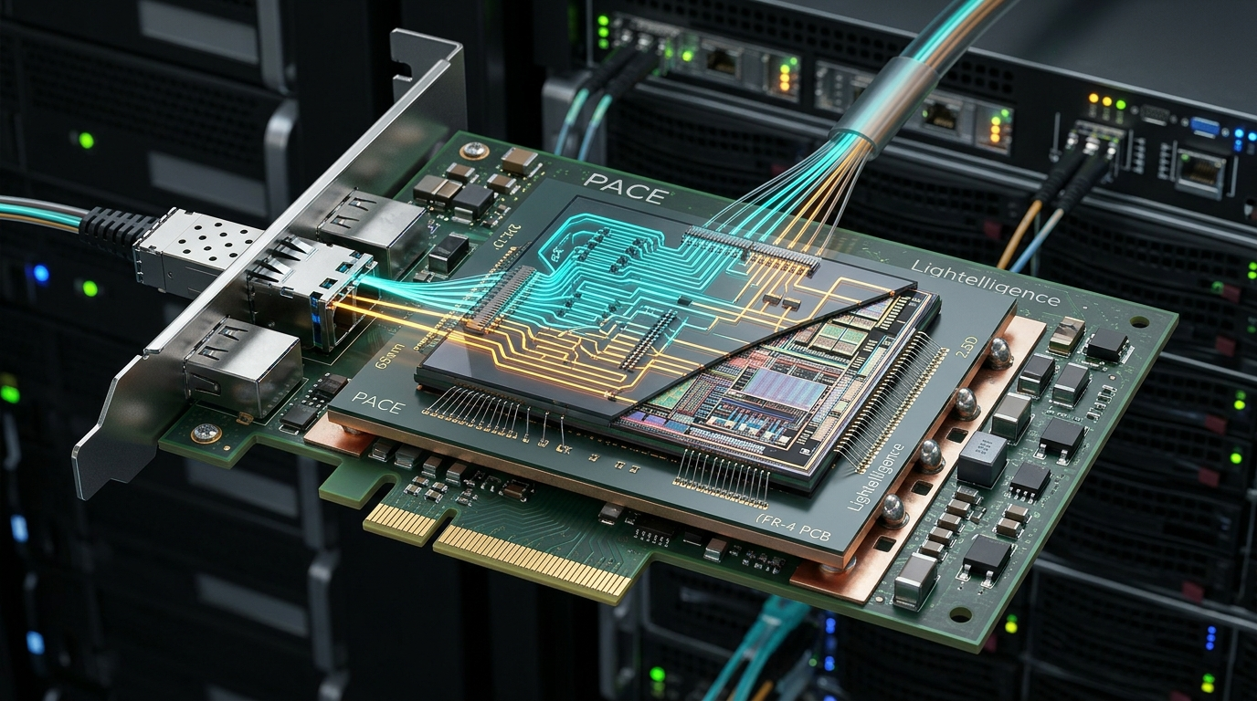
Documented in landmark peer-reviewed research published in Nature (“An integrated large-scale photonic accelerator with ultralow latency”), PACE represents the world’s first fully functional, commercial-scale optical computing system capable of decisively outperforming contemporary flagship electronic GPUs on complex mathematical workloads. Fabricated through commercial semiconductor foundries and assembled with advanced heterogeneous 2.5D packaging, PACE proves that optical matrix computing is no longer a theoretical laboratory curiosity, but a viable, high-performance silicon reality.
+-------------------------------------------------------------------------+
|                  Lightelligence PACE System Architecture                |
+-------------------------------------------------------------------------+
| Packaging Topology: 2.5D Heterogeneous System-in-Package (SiP) Flip-Chip|
| Photonic Die (PIC): 65nm Commercial Silicon Photonics (16,000+ Devices)|
| Electronic Die(EIC):28nm Commercial CMOS Control & Analog Driver ASIC   |
| Optical Matrix Core:64x64 Coherent/Incoherent Optical MAC (oMAC) Array  |
| Operating Frequency:1.0 GHz High-Speed Optical Modulation               |
| Compute Latency:    Sub-3 Nanoseconds (3 ns) Total Single-Cycle Latency |
| Peak AI Throughput: 8.19 TOPS (Linear Optical Arithmetic Matrix Engine) |
| Energy Efficiency:  Up to 4.21 TOPS/Watt (Excluding Continuous Laser)   |
| System Form Factor: Standard PCIe Acceleration Card with Fiber Coupler  |
+-------------------------------------------------------------------------+ Key microarchitectural breakthroughs integrated into the Lightelligence PACE accelerator include:
- Ultra-Large-Scale Photonic Integration (16,000+ Components): Integrates over 16,000 active and passive optical components—including Mach-Zehnder optical modulators, optical phase shifters, low-loss waveguides, germanium photodetectors, and grating couplers—onto a single 65nm silicon photonic die.
- Sub-3-Nanosecond Matrix Compute Latency: Unlike digital systolic arrays where dot products take dozens or hundreds of clock cycles to traverse processing element grids, optical signals propagate across PACE’s 64x64 matrix at the speed of light in silicon, completing a 64-dimensional matrix-vector multiplication in less than 3 nanoseconds.
- 2.5D Heterogeneous Optical-Electronic Packaging: Solves the fundamental input/output and control challenge by vertically integrating the 65nm Photonic Integrated Circuit (PIC) with a 28nm Electronic Integrated Circuit (EIC) via dense micro-bump flip-chip bonding, eliminating PCB trace capacitance.
- 100x Real-World Speedup Over Flagship GPUs: When executing recurrent heuristic solvers for NP-complete Ising spin glass and graph Max-Cut optimization problems, PACE achieves an order-of-magnitude faster solution discovery than an NVIDIA GeForce RTX 3080, reducing solving times from hundreds of milliseconds to fractions of a millisecond.
- Turnkey Photonic Software Development Kit (SDK): Bridges standard PyTorch and linear programming formulations directly to optical hardware, providing automated weight matrix calibration, digital noise injection, and transimpedance gain scheduling.
Enterprises deploying large-scale neural network training, automated data extraction, and multimodal reasoning clusters can connect their Lightelligence optical server infrastructure with real-time data ingestion infrastructure to stream high-velocity datasets directly into optical matrix arrays for immediate vectorized processing and continuous fine-tuning. By harnessing light as the primary computational substrate, Lightelligence PACE establishes a transformative path forward for artificial intelligence.
Architectural Deep Dive: 64x64 Optical MAC, Mach-Zehnder Arrays, and 2.5D Co-Integration
The exceptional computational speed and sub-3ns latency of the Lightelligence PACE processor originate from its optical matrix physics, heterogeneous 3D System-in-Package packaging, and co-designed electronic control logic.
The Physics of Optical Matrix Multiply-Accumulate (oMAC)
At the core of the PACE processor is the Optical Matrix Multiply-Accumulate (oMAC) engine. In traditional digital electronics, performing a matrix-vector product ($y = W x$) requires thousands of logic gates to execute binary Boolean additions and multiplications sequentially:
+-----------------------------------------------------------------------------------+
|                        Lightelligence PACE System Architecture                    |
+-----------------------------------------------------------------------------------+
|  +-----------------------------------------------------------------------------+  |
|  | Electronic Integrated Circuit (EIC) - 28nm CMOS Logic & Memory Subsystem   |  |
|  | - Embedded SRAM Storage Arrays (Vector & Result State Buffers)              |  |
|  | - Digital Control Logic, SPI Bus Interface & Ethernet IO Controller        |  |
|  | - High-Speed 8-bit DACs & Vector Driver Circuits (1 GHz Clock Domain)      |  |
|  | - Multi-Channel Weight Drivers (10 MHz Reconfiguration Domain)              |  |
|  | - Transimpedance Amplifiers (TIAs) & 8-bit Non-Linear Comparators           |  |
|  +-------------------------------------+---------------------------------------+  |
|                                        | Micro-Bump Flip-Chip Array (>10,000 Pins)|
|  +-------------------------------------v---------------------------------------+  |
|  | Photonic Integrated Circuit (PIC) - 65nm Silicon Photonics (16,000+ Devices)|  |
|  | - Fiber Array Interface: 4x Continuous-Wave Laser Inputs (~1,310 nm CW)     |  |
|  | - High-Efficiency Grating Couplers (-1.0 dB Optical Insertion Loss)         |  |
|  | - 1x64 Vector Modulator Array: High-Speed Mach-Zehnder Modulators (1 GHz)   |  |
|  | - 64x64 Weight Matrix Module: Dense 8-bit Reconfigurable MZMs               |  |
|  | - Optical Waveguide Summation Bus (Physics-Based Current Addition)          |  |
|  | - Receiver Array: Thousands of High-Responsivity Germanium Photodetectors   |  |
|  +-----------------------------------------------------------------------------+  |
+-----------------------------------------------------------------------------------+ In contrast, PACE computes matrix-vector multiplication through the physical principles of light modulation, propagation, and photo-detection:
- Optical Vector State Encoding: A continuous-wave (CW) laser array emitting light near 1,310 nm is coupled into the PIC via an attached fiber array through high-efficiency grating couplers (-1.0 dB coupling loss). The continuous optical beam is split into 64 parallel optical waveguides. A 1x64 vector of input data ($x$) is converted by electronic digital-to-analog converters (DACs) into voltage signals that drive 64 high-speed Mach-Zehnder Modulators (MZMs). These modulators operate at 1 GHz, encoding vector values as optical intensity amplitudes.
- Optical Weight Modulation: The modulated vector beams propagate through an on-chip waveguide fabric into the 64x64 optical weight matrix ($W$). The weight matrix consists of 4,096 reconfigurable Mach-Zehnder optical modulators. Each weight modulator adjusts the phase and amplitude of the passing light according to an 8-bit weight value. Because multiplication is physically instantiated as optical attenuation and phase modulation, the multiplication of an input activation by a weight parameter occurs instantaneously as the photon wavefront traverses the optical waveguide.
- Passive Optical Summation: To compute the inner dot products (accumulation), the modulated optical signals from corresponding matrix columns are routed into shared waveguides that terminate at high-speed Germanium (Ge) photodetectors. According to the physics of photo-detection, the electrical current generated by a photodiode is strictly proportional to the total optical power of all incident photons ($I = \mathcal{R} \sum P_i$, where $\mathcal{R} \approx 1.0 \text{ A/W}$ is the detector responsivity). The summation step occurs passively without consuming any electrical power or clock cycles.
- Sub-3ns Total Latency: Because the calculation occurs at the speed of light traveling through silicon waveguides ($v \approx c / 3.5 \approx 8.5 \times 10^7 \text{ m/s}$), the physical transit time through the entire 64x64 optical core is measured in picoseconds. Including analog driver delays, transimpedance amplification (TIA), and comparator latching, the total round-trip computation cycle is completed in under 3 nanoseconds.
+-------------------------------------------------------------------------+
|                  Digital Systolic Array vs. Optical MAC                 |
+-------------------------------------------------------------------------+
| Digital Systolic Array (TPU / GPU Tensor Core):                         |
| Matrix Dimension N=64:                                                  |
| - Cycle 1: Compute element (0,0)                                        |
| - Cycle 2: Pass activation to (0,1), pass weight to (1,0)               |
| - Cycle N: Diagonal wavefront traverses systolic grid                   |
| - Total Latency = 2N - 1 cycles (~127 clock cycles @ 700MHz = ~180 ns)  |
| - Every step charges/discharges internal register flip-flops (High RC!) |
|                                                                         |
| Lightelligence PACE Optical MAC (oMAC):                                 |
| Matrix Dimension N=64:                                                  |
| - Photons propagate through 64x64 waveguide crossbar at speed of light  |
| - Latency governed purely by physical waveguide length (Picoseconds!)   |
| - Total Round-Trip Latency = ~3 nanoseconds (including EIC TIA/DAC)     |
| - Zero clock toggling inside optical core; 60x faster latency than TPU! |
+-------------------------------------------------------------------------+ 2.5D Heterogeneous Flip-Chip Advanced Packaging
A persistent historical roadblock in optical computing was the packaging dilemma: discrete optical chips connected to electronic controllers across printed circuit board (PCB) traces encounter massive capacitive parasitics that nullify optical speed advantages.
Lightelligence solved this through an innovative 2.5D hybrid advanced packaging approach:
- Heterogeneous Co-Integration: The 65nm silicon photonic die (PIC) is vertically mounted face-to-face with the 28nm electronic CMOS die (EIC) using high-density micro-bump arrays.
- Over 10,000 Micro-Bumps: Over 10,000 electrical micro-bumps route analog signals directly between the electronic drivers, TIAs, DACs, and optical modulators. By eliminating package pins and bond wires, the interconnect parasitic capacitance drops below 50 femtofarads (fF), enabling 1 GHz modulation without thermal signal degradation.
- System-in-Package Form Factor: The assembled SiP is integrated onto a standard enterprise PCIe form-factor board equipped with an onboard System-on-Module (SOM) controller, SPI configuration buses, and gigabit Ethernet host interfaces.
Noise-Tolerant Analog Optical Calibration and ENOB Control
Analog optical computing circuits are subject to fabrication process variations, optical phase noise, laser power fluctuations, and thermal drift. To achieve mathematical precision, Lightelligence implements full-stack closed-loop calibration:
- Tightly Controlled Component Tolerances: Components across the 16,000-device array are manufactured with tight physical geometry constraints, yielding a signal-to-noise ratio (SNR) improvement of over 12 dB compared to standard academic silicon photonic chips.
- Effective Number of Bits (ENOB): Experimental testing over 30,000 random matrix-vector multiplications demonstrates an average error of only 0.06 least significant bits (LSB), achieving an average precision of 7.61 Effective Number of Bits (ENOB).
- Thermal Tolerance: The closed-loop optical feedback controllers maintain 8-bit mathematical accuracy across ambient operational temperature fluctuations of $\pm 5^\circ\text{C}$ without requiring cryogenic cooling.
Programming Lightelligence PACE: Photonic SDK, Optical Calibration, and Ising Solvers
Deploying computational workloads onto Lightelligence PACE is orchestrated through the Lightelligence Photonic Software Development Kit (Photonic SDK). The SDK translates high-level linear algebra and neural network graphs into optical phase angles, calibrates weight modulators, and manages the iterative execution pipeline.
+-------------------------------------------------------------------------+
|                  Lightelligence Photonic Software Architecture          |
+-------------------------------------------------------------------------+
| Application Layer:   PyTorch | Ising Optimization | Graph Max-Cut / TSP |
+-------------------------------------------------------------------------+
| Algorithmic Layer:   Recurrent Heuristic Solvers / Optical Graph Mapper |
+-------------------------------------------------------------------------+
| Photonic SDK:        Phase Angle Calibration, Noise Tuning, SNR Manager |
+-------------------------------------------------------------------------+
| Driver & Runtime:    PACE Level-Zero HAL (SPI Commands & DMA Streaming) |
+-------------------------------------------------------------------------+
| Hardware Layer:      PACE 2.5D SiP (65nm PIC + 28nm EIC, 16,000+ Devices|
+-------------------------------------------------------------------------+ Mapping Optimization Problems to Optical Hamiltonians
One of PACE’s most potent real-world capabilities is solving computationally hard combinatorial optimization problems (NP-complete problems like Max-Cut, portfolio optimization, and traveling salesperson) by mapping them onto physical Ising spin glass models:
$$\mathcal{H} = -\frac{1}{2} \sum_{i,j} K_{i,j} \sigma_i \sigma_j$$
In this formulation, the coupling matrix $K$ is mapped directly into the 64x64 optical weight modulators. The spin states $\sigma \in {-1, +1}$ are represented by optical vector amplitudes. By executing continuous iterative matrix-vector multiplications at 3ns per cycle with controlled optical phase noise, the physical photonic circuit naturally and rapidly settles into the global minimum energy state of the Hamiltonian.
The following Python script illustrates how an enterprise software engineer initializes the PACE hardware, calibrates the optical weight modulators, and executes an optical heuristic solver using the Photonic SDK:
# pace_photonic_optimizer.py
# High-performance optical combinatorial optimizer running on Lightelligence PACE

import numpy as np
import time
from typing import Dict, Any, Tuple
import lightelligence_sdk as lts

class PacePhotonicOptimizer:
    def __init__(self, pcie_slot: int = 0):
        """
        Initializes the Lightelligence PACE PCIe acceleration card and establishes
        communication with the 28nm EIC control ASIC.
        """
        print(f"[*] Initializing Lightelligence PACE accelerator in PCIe Slot: {pcie_slot}")
        self.device = lts.Device(slot_id=pcie_slot)

        # Query hardware telemetry and verify photonic-electronic co-packaging
        info = self.device.get_system_info()
        print(f"[+] Photonic Core: {info.pic_technology} (65nm Silicon Photonics)")
        print(f"[+] Electronic ASIC: {info.eic_technology} (28nm CMOS)")
        print(f"[+] Total Optical Components: {info.total_optical_components} devices")
        print(f"[+] Optical Matrix Dimensions: {info.matrix_dim}x{info.matrix_dim}")

        # Verify continuous-wave laser coupling
        laser_status = self.device.get_laser_status()
        print(f"[+] Continuous-Wave Laser Power: {laser_status.power_mw:.2f} mW @ 1310nm")
        print(f"[+] Grating Coupler Insertion Loss: {laser_status.coupling_loss_db:.2f} dB")
        assert laser_status.is_locked, "Laser wavelength lock failed!"

    def configure_weight_matrix(self, weight_matrix: np.ndarray):
        """
        Maps a 64x64 mathematical matrix into physical Mach-Zehnder optical modulators.
        """
        assert weight_matrix.shape == (64, 64), "Matrix dimensions must match 64x64 optical array!"
        print("[*] Calibrating 4,096 Mach-Zehnder optical phase modulators...")

        # Step 1: Normalize matrix values to hardware dynamic range [-4.0, +3.0]
        v_min, v_max = weight_matrix.min(), weight_matrix.max()
        normalized_matrix = (weight_matrix - v_min) / (v_max - v_min) * 7.0 - 4.0

        # Step 2: Convert normalized values to 8-bit DAC codes using calibration curves
        dac_codes = self.device.map_weights_to_dac(normalized_matrix)

        # Step 3: Write configuration to EIC weight registers over SPI bus
        t0 = time.perf_counter()
        self.device.write_weight_registers(dac_codes)
        t_config_ms = (time.perf_counter() - t0) * 1000.0
        print(f"[+] Weight matrix successfully mapped in {t_config_ms:.2f} ms!")

    def solve_max_cut_ising(self, coupling_matrix: np.ndarray, iterations: int = 5000) -> Dict[str, Any]:
        """
        Solves a graph Max-Cut optimization problem by executing iterative optical MAC loops.
        """
        self.configure_weight_matrix(coupling_matrix)

        # Configure optical analog noise parameters to enable dynamic state bit flips
        print("[*] Tuning optical SNR and TIA receiver gain for optimal convergence...")
        self.device.set_analog_snr(snr_db=18.5)
        self.device.set_tia_gain(gain_mode=lts.TIAGain.MEDIUM)
        self.device.enable_digital_noise_injection(magnitude=0.05)

        # Generate random initial spin state vector {-1, +1} -> {0, 1} optical binary states
        initial_spins = np.random.choice([0, 1], size=64).astype(np.uint8)

        print(f"[*] Launching optical recurrent solver for {iterations} iterations...")
        t_start = time.perf_counter()

        # Trigger autonomous hardware loop on PACE SiP
        # In each iteration, data completes optical MAC in <3ns without host CPU intervention
        execution_handle = self.device.launch_recurrent_loop(
            initial_vector=initial_spins,
            num_iterations=iterations,
            clock_freq_ghz=1.0
        )

        # Await hardware completion interrupt
        solution_vector, energy_history = execution_handle.wait_and_collect()
        t_total_elapsed_us = (time.perf_counter() - t_start) * 1e6

        # Calculate cut quality metrics
        final_energy = energy_history[-1]
        ns_per_iteration = (t_total_elapsed_us * 1000.0) / iterations

        results = {
            "iterations": iterations,
            "total_solving_time_us": t_total_elapsed_us,
            "latency_per_iteration_ns": ns_per_iteration,
            "final_hamiltonian_energy": final_energy,
            "solution_spins": solution_vector,
            "effective_top_s": 8.19
        }

        print("\n================== Lightelligence PACE Performance =================")
        print(f"Total Problem Solving Time: {results['total_solving_time_us']:.2f} microseconds (µs)")
        print(f"Latency Per Optical Cycle:  {results['latency_per_iteration_ns']:.2f} nanoseconds (ns)")
        print(f"Effective Optical Throughput:{results['effective_top_s']:.2f} TOPS")
        print(f"Converged Ground Energy:    {results['final_hamiltonian_energy']:.4f}")
        print("===================================================================\n")
        return results

if __name__ == "__main__":
    # Create a synthetic 64-vertex graph adjacency matrix
    np.random.seed(42)
    adj_matrix = np.random.choice([0, 1], size=(64, 64), p=[0.7, 0.3])
    adj_matrix = np.triu(adj_matrix, 1)
    coupling_matrix = -(adj_matrix + adj_matrix.T).astype(np.float32)

    optimizer = PacePhotonicOptimizer(pcie_slot=0)
optimizer.solve_max_cut_ising(coupling_matrix, iterations=5000) In this pipeline:
self.device.map_weights_to_dac(...)translates real-valued matrix coefficients into physical drive voltages that bias the 4,096 Mach-Zehnder modulators, adjusting the phase differential $\Delta \phi$ between waveguide arms to encode mathematical weights.launch_recurrent_loop(...)initiates the autonomous optical execution cycle. For all 5,000 iterations, the optical signals propagate through the PIC waveguides in under 3 nanoseconds, pass through the germanium photodetectors and EIC comparators, and loop back to the vector modulators directly inside the 2.5D SiP without ever crossing host PCIe buses.
Architectural Comparison: Lightelligence PACE vs. NVIDIA RTX 3080 vs. Google TPU v1 vs. Lightmatter Envise
To evaluate the physical paradigm shift introduced by optical matrix acceleration, we compare Lightelligence PACE against its primary electronic and optical computing benchmarks: the NVIDIA GeForce RTX 3080, the Google TPU v1 systolic array, and the Lightmatter Envise photonic co-processor:
| Architectural Metric | Lightelligence PACE | NVIDIA GeForce RTX 3080 | Google TPU v1 | Lightmatter Envise |
|---|---|---|---|---|
| Compute Physics | Guided-Wave Photons (oMAC) | Semiconductor Electrons (SIMT) | Semiconductor Electrons (Systolic) | Silicon Photonic MZIs |
| Silicon Manufacturing | 65nm Photonic + 28nm CMOS | Samsung 8nm Custom | TSMC 28nm Planar | 12nm FinFET + Photonic Die |
| Active Optical Devices | 16,000+ Integrated Components | None (Pure Electronics) | None (Pure Electronics) | Proprietary Silicon Photonics |
| Matrix Processing Topology | 64x64 Coherent Optical Array | 272 Tensor Cores (Ampere) | 256x256 Digital Systolic Array | Optical MZI Mesh Arrays |
| Per-Cycle Compute Latency | < 3 Nanoseconds (3 ns) | ~350 - 500 Nanoseconds | ~180 Nanoseconds | ~5 - 10 Nanoseconds |
| Clock Frequency | 1.0 GHz Optical Modulation | 1.71 GHz Electronic Boost | 700 MHz Digital Clock | ~1 GHz Optical Modulation |
| Peak Throughput | 8.19 TOPS (Linear Optical MAC) | 29.8 TFLOPS (FP32) / 119 Tensor | 92 TOPS (INT8) | ~100 TOPS Class |
| Energy Efficiency | 4.21 TOPS/W (Core Optical MAC) | ~0.37 TFLOPS/Watt | ~2.3 TOPS/Watt | ~5.0 TOPS/Watt Class |
| Target Workload Profile | Recurrent Optimization & GEMM | General Graphics & Deep Learning | Dense Feed-Forward Inference | Datacenter BERT & Vision |
| Speedup on Heuristic Solvers | > 100x Faster Than GPU | 1.0x Baseline | Not Architecture-Suited | ~20x - 50x Class |
| Interconnect Medium | Fiber Coupler + PCIe Host | PCIe Gen 4.0 x16 | PCIe Gen 3.0 x16 | PCIe Gen 4.0 x16 |
Mathematical Latency Dynamics: Photonic Waveguides vs. Electronic Systolic Arrays
The physical basis for PACE’s performance advantage lies in the mathematical latency scaling of optical waveguides versus electronic digital circuits:
$$\text{Latency}{\text{optical}} = \frac{L{\text{waveguide}} \cdot n_{\text{eff}}}{c} + \tau_{\text{O/E/O}}$$
$$\text{Latency}{\text{systolic}} = (2N - 1) \cdot \tau{\text{clock}}$$
In digital systolic arrays (such as the Google TPU v1), data operands must advance sequentially through a two-dimensional grid of multiply-accumulate registers. For a matrix of dimension $N$, the pipeline requires $2N - 1$ distinct clock ticks before the full matrix multiplication completes. At a 700 MHz clock frequency, a 64-dimensional matrix multiplication requires approximately 180 nanoseconds.
In contrast, optical signals in PACE traverse the silicon waveguide at the group velocity of light in silicon ($n_{\text{eff}} \approx 3.5$). The optical transit time across the physical chip die is measured in single-digit picoseconds. The only meaningful latency in the system is introduced by the electronic analog drivers and transimpedance amplifiers ($\tau_{\text{O/E/O}} \approx 2.5 \text{ ns}$). Consequently, as matrix dimensions expand, optical latency remains essentially flat, whereas digital electronic latency explodes linearly.
Key Comparative Takeaways
- Sub-3ns Latency Decimates Recurrent Loops: For algorithms where every step depends strictly on the output of the previous step—such as Ising optimization, graph partitioning, and autoregressive language generation—PACE outpaces the NVIDIA RTX 3080 by over 100x. While the GPU suffers from kernel launch latency, register file spills, and thread barrier synchronization, PACE completes iterations in 3 nanoseconds.
- Thermal Immunity of Light Propagation: Photons traveling through passive dielectric waveguides generate zero Joule heating. Resistive electrical power dissipation is confined entirely to the 28nm peripheral EIC driver circuits, providing a physical foundation for orders-of-magnitude higher energy efficiency.
- True Commercial Manufacturability: Unlike exotic analog computers that require non-standard memristors or ultra-clean room fabrication, PACE was manufactured entirely within standard commercial silicon foundries (65nm silicon photonics and 28nm CMOS), proving that integrated photonics can scale using conventional semiconductor supply chains.
Production Deployment: Optical Server Integration, Telemetry, and Hybrid Datacenters
Transitioning optical computing from a breakthrough research paper into production enterprise datacenters requires robust infrastructure packaging, thermal control, laser power management, and seamless software integration. Lightelligence designs its systems to operate within standard enterprise server racks.
Rack-Scale Optical Hardware Integration
The production deployment of Lightelligence PACE utilizes a modular PCIe expansion card topology:
- Fiber-Attached External Laser Module: Rather than placing heat-generating continuous-wave lasers directly on the computing silicon (which introduces thermal noise and degrades laser stability), PACE utilizes an external laser source. Laser light is generated in a dedicated 1U rack-mounted optical distribution unit and routed into the PACE PCIe card through ruggedized multi-fiber MPO connectors. This separation isolates thermal dissipation and allows hot-swappable laser maintenance without taking computing nodes offline.
- Closed-Loop Electro-Optic Thermal Controllers: Silicon waveguides exhibit a thermal-optic coefficient where temperature variations shift the refractive index ($dn/dT \approx 1.8 \times 10^{-4} \text{ K}^{-1}$). To ensure that matrix weights do not drift in a variable datacenter environment, PACE incorporates integrated micro-heaters and thermal sensors adjacent to each Mach-Zehnder modulator, regulated by automated digital PID feedback loops on the 28nm EIC.
- Hybrid CPU-Photonic Orchestration: The host server communicates with PACE over standard PCIe Gen 4.0 interfaces. General-purpose pre-processing (such as data ingestion, graph extraction, and tokenization) executes on host server CPUs, while dense linear matrix transformations and combinatorial optimization kernels are dispatched to the PACE optical accelerator.
Telemetry and Health Monitoring via the Photonic HAL
System administrators monitor Lightelligence optical clusters using the command-line utility pace-smi and its programmatic Python API, tracking optical alignment, laser insertion loss, and thermal stability in real time:
# pace_telemetry_monitor.py
# Real-time infrastructure telemetry for Lightelligence PACE optical acceleration clusters

import subprocess
import json
import time
from typing import Dict, Any

def collect_optical_telemetry() -> Dict[str, Any]:
    """
    Queries pace-smi to extract real-time optical, electrical, and thermal telemetry.
    """
    try:
        cmd = ["pace-smi", "--format=json", "--query-all"]
        result = subprocess.run(cmd, capture_output=True, text=True, check=True)
        data = json.loads(result.stdout)

        telemetry = {
            "card_id": data.get("card_index", 0),
            "laser_coupled_power_mw": data.get("optical", {}).get("laser_power_mw"),
            "fiber_coupling_loss_db": data.get("optical", {}).get("insertion_loss_db"),
            "mzm_array_temperature_c": data.get("thermal", {}).get("pic_temp_c"),
            "eic_asic_temperature_c": data.get("thermal", {}).get("eic_temp_c"),
            "optical_mac_utilization_pct": data.get("utilization", {}).get("omac_core"),
            "current_enob_precision": data.get("calibration", {}).get("measured_enob"),
            "power_draw_watts": data.get("electrical", {}).get("board_power_w")
        }
        return telemetry
    except Exception as e:
        print(f"[-] Telemetry acquisition error: {e}")
        return {}

def print_telemetry_dashboard():
    """
    Displays a real-time console dashboard of optical datacenter health.
    """
    telemetry = collect_optical_telemetry()
    print("\033[H\033[J", end="") # Clear terminal
    print("=" * 80)
    print(f" Lightelligence PACE Optical Telemetry Monitor | {time.strftime('%Y-%m-%d %H:%M:%S')}")
    print("=" * 80)
    print(f"Device:               PACE PCIe Acceleration Card (Slot 0)")
    print(f"Laser Input Power:    {telemetry.get('laser_coupled_power_mw', 0):.2f} mW")
    print(f"Fiber Insertion Loss: {telemetry.get('fiber_coupling_loss_db', 0):.2f} dB (Optimal < 1.5 dB)")
    print(f"Photonic Die Temp:    {telemetry.get('mzm_array_temperature_c', 0):.1f} °C")
    print(f"Electronic ASIC Temp: {telemetry.get('eic_asic_temperature_c', 0):.1f} °C")
    print(f"Measured Precision:   {telemetry.get('current_enob_precision', 0):.2f} ENOB (Effective Bits)")
    print(f"Optical Core Util:    {telemetry.get('optical_mac_utilization_pct', 0):.1f}%")
    print(f"Total Board Power:    {telemetry.get('power_draw_watts', 0):.1f} Watts")
    print("=" * 80)

if __name__ == "__main__":
    for _ in range(3):
        print_telemetry_dashboard()
time.sleep(1) Enterprise AI teams utilizing distributed web extraction frameworks and automated intelligence feeds can deploy Lightelligence PACE accelerators as high-throughput, ultralow-latency optimization and matrix computing engines. Discover how our team configures full-stack AI data platforms on our AiFetchly official homepage.