LGM Guide: High-Resolution 3D Gaussian Splatting Generation
The 3D Rendering Dilemma: The Limits of NeRF Volumetric Ray-Marching
In modern digital commerce, spatial simulation, real-time gaming, and automated web intelligence pipelines powered by AiFetchly, generative artificial intelligence has expanded rapidly from flat 2D images and video into interactive three-dimensional geometry. Enterprise systems increasingly demand automated 3D asset creation: turning single product catalog photographs into interactive 3D digital twins, generating assets for gaming environments, and creating physical representations for robotics simulation.
However, existing 3D generative foundation models—primarily grounded in Neural Radiance Fields (NeRF) and triplane representations (such as LRM or TripoSR)—collide with severe rendering bottlenecks:
The 3D Neural Rendering Bottlenecks:
+-----------------------------------------------------------------------------------+
| 1. The Volumetric Ray-Marching Tax                                                |
| • NeRF queries continuous 3D points via volumetric ray-marching                   |
| • Requires sampling 64 to 256 coordinates per individual screen pixel             |
| X Extremely slow rendering latency: 0.5 to 2.0 seconds per novel view image!      |
| X Prohibitive for real-time interactive 60 FPS viewports and WebGL engines!       |
+-----------------------------------------------------------------------------------+
| 2. Low-Resolution Training Supervision Bottleneck                                 |
| • Training NeRFs at 512x512 resolution exhausts GPU High-Bandwidth Memory (HBM)   |
| • Prior models are restricted to supervising at 64x64 or 128x128 resolution       |
| X Results in blurry surface textures, missing thin geometries, and specular drift!|
+-----------------------------------------------------------------------------------+
| 3. Mesh Polygonization Artifacts (Marching Cubes Flaws)                           |
| • Converting volumetric NeRF density grids into polygon meshes (.obj) introduces  |
|   topological noise, jagged edges, disconnected floating floaters, and loss of detail|
| X Requires expensive manual 3D cleanup before assets can be rendered in engines!  |
+-----------------------------------------------------------------------------------+ 1. The Computational Cost of Volume Rendering
The core mathematical primitive of NeRF is the continuous volume rendering integral along camera rays $\mathbf{r}(t) = \mathbf{o} + t\mathbf{d}$:
$$C(\mathbf{r}) = \int_{t_n}^{t_f} T(t) \sigma(\mathbf{r}(t)) \mathbf{c}(\mathbf{r}(t), \mathbf{d}) , dt, \quad \text{where } T(t) = \exp\left(-\int_{t_n}^t \sigma(\mathbf{r}(s)) , ds\right)$$
To evaluate this integral numerically for a single $512 \times 512$ viewport image:
- The GPU must cast 262,144 camera rays.
- Each ray samples between 64 and 128 discrete 3D spatial points.
- This requires over 25 million MLP evaluations per frame.
- Consequently, novel-view synthesis runs at merely 1 to 5 frames per second on high-end GPUs, making smooth, interactive inspection in web browsers or mobile apps completely infeasible.
2. The Resolution Ceiling in Feed-Forward Training
In feed-forward 3D generative architectures (such as Large Reconstruction Models):
- Computing volume rendering across multiple camera views during training is extraordinarily memory-intensive.
- Backpropagating gradients through millions of ray-sampled points forces models to downsample supervision images to $64 \times 64$ or $128 \times 128$ resolution.
- As a consequence, models struggle to learn fine-grained high-frequency details, such as intricate mechanical parts, crisp text labels on packaging, or specular reflections on metal and glass surfaces harvested via AiFetchly Web Scraping.
3. The 3D Gaussian Splatting Alternative
In 2023, Kerbl et al. revolutionized novel view synthesis with 3D Gaussian Splatting (3D-GS):
- 3D-GS replaces continuous volumetric fields with an explicit collection of anisotropic 3D Gaussian ellipsoids.
- Gaussians are projected onto 2D image planes and rendered using differentiable tile-based rasterization, achieving blazing-fast rendering speeds exceeding 100+ FPS at 1080p resolution.
- However, standard 3D-GS requires per-scene optimization: fitting Gaussians to an object takes 10 to 30 minutes of gradient descent per scene.
- Can we build a foundation model that directly predicts complete 3D Gaussian Splats in a single feed-forward forward pass?
The Solution: LGM Architecture & Asymmetric U-Net
To bring the real-time rendering speed and fidelity of 3D Gaussian Splatting into feed-forward foundation models, researchers from Peking University, S-Lab NTU, and Shanghai AI Lab (Tang et al., ECCV 2024 oral) introduced LGM: Large Multi-View Gaussian Model for High-Resolution 3D Content Creation.
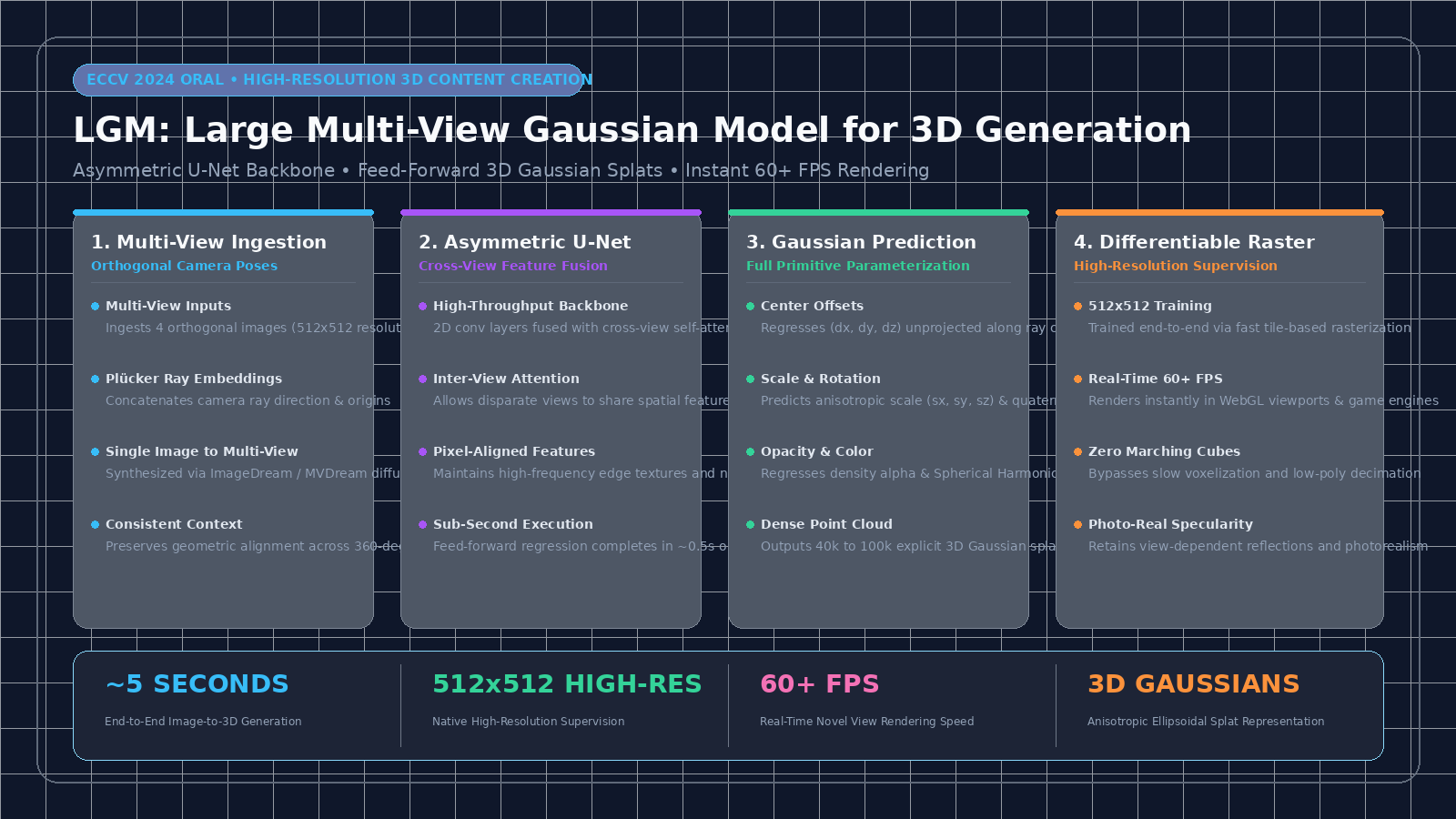
LGM is a generalist 3D foundation model that takes multi-view images of an object (typically 4 orthogonal views generated from text or a single photograph) and directly regresses a dense cloud of over 40,000 to 100,000 3D Gaussians in a single feed-forward pass executing in ~0.5 seconds on an NVIDIA RTX 3090/4090.
The LGM Feed-Forward Architecture:
+---------------------------------------------------------------------------------------------------+
| 1. MULTI-VIEW CAMERA & RAY CONCATENATION                                                          |
| Input: 4 Multi-View RGB Images at 512x512 resolution (generated via ImageDream / MVDream)         |
| Concatenated with Plücker Ray Embeddings (Ray Origins o and Normalized Directions d)               |
| Input Tensor Shape: (Batch, 4 Views, 9 Channels, 512, 512)                                        |
+---------------------------------------------------------------------------------------------------+
                                                  |
                                                  v
+---------------------------------------------------------------------------------------------------+
| 2. ASYMMETRIC U-NET WITH CROSS-VIEW ATTENTION                                                     |
| • 2D Convolutional Encoder & Decoder preserves high-resolution pixel spatial priors               |
| • Inter-View Self-Attention layers allow cross-camera feature exchange across all 4 views         |
| • Scales efficiently: eliminates expensive 3D voxelization or quadratic 3D transformer tokens     |
+---------------------------------------------------------------------------------------------------+
                                                  |
                                                  v
+---------------------------------------------------------------------------------------------------+
| 3. PIXEL-ALIGNED 3D GAUSSIAN REGRESSION HEAD                                                      |
| For every pixel in each view, the network predicts 14 primitive parameters:                       |
| • Position Center Offset: Delta p in R^3 (unprojected along Plücker ray)                          |
| • Anisotropic Scale: s = (s_x, s_y, s_z) in R^3 (log-space positive scale)                        |
| • Rotation Quaternion: q = (q_w, q_x, q_y, q_z) in R^4 (L2-normalized)                           |
| • Opacity: alpha in [0, 1] (via Sigmoid activation)                                               |
| • Spherical Harmonics Color: c in R^3 (RGB base coefficients)                                     |
| Output: Dense cloud of ~40k - 100k fully parameterized 3D Gaussians!                              |
+---------------------------------------------------------------------------------------------------+
                                                  |
                                                  v
+---------------------------------------------------------------------------------------------------+
| 4. DIFFERENTIABLE TILE RASTERIZATION & HIGH-RESOLUTION SUPERVISION                                |
| • Renders arbitrary novel views at 512x512 resolution in <5ms using fast CUDA tile rasterizer     |
| • Supervised directly with L1 photometric loss + LPIPS perceptual loss on high-res ground truth   |
| • Delivers instant 60+ FPS interactive WebGL rendering with zero mesh polygonization artifacts!   |
+---------------------------------------------------------------------------------------------------+ 1. Plücker Ray Coordinate Conditioning
To ensure the network understands camera geometry across disparate view angles without coordinate drift:
-
Each pixel $(u, v)$ in view $v_k$ is augmented with its corresponding camera ray using Plücker coordinates:
$$\mathbf{r} = (\mathbf{d}, \mathbf{o} \times \mathbf{d}) \in \mathbb{R}^6$$
where $\mathbf{o} \in \mathbb{R}^3$ is the camera optical center and $\mathbf{d} \in \mathbb{R}^3$ is the normalized ray direction.
-
The 3-channel RGB image is concatenated with the 6-channel Plücker ray representation, creating a 9-channel input tensor per view: $\mathbf{X}_{\text{in}} \in \mathbb{R}^{B \times 4 \times 9 \times 512 \times 512}$.
2. High-Throughput Asymmetric U-Net
Rather than using computationally heavy 3D transformers (which struggle with dense $512 \times 512$ inputs), LGM adopts a high-throughput Asymmetric 2D U-Net backbone:
- 2D Convolutional Strides: Convolutions excel at processing high-resolution local features (edges, textures, surface reflections) with linear memory complexity $O(HW)$.
- Inter-View Cross-Attention: At intermediate downsampled feature stages (e.g., $64 \times 64$ and $32 \times 32$), LGM inserts multi-head self-attention layers that operate across the 4 camera viewpoints:
- Tokens at view $k$ attend to tokens from the remaining three views.
- This cross-view communication resolves occlusion boundaries and enforces 3D consistency between front, side, and rear surfaces.
3. Pixel-Aligned 3D Gaussian Primitive Parameterization
Each 3D Gaussian primitive $\mathcal{G}_i$ is defined by:
$$G(\mathbf{x}) = \exp\left(-\frac{1}{2} (\mathbf{x} - \boldsymbol{\mu}_i)^\top \boldsymbol{\Sigma}_i^{-1} (\mathbf{x} - \boldsymbol{\mu}_i)\right)$$
The covariance matrix $\boldsymbol{\Sigma}_i$ is parameterized by an anisotropic scaling vector $\mathbf{s}_i \in \mathbb{R}^3$ and a rotation quaternion $\mathbf{q}_i \in \mathbb{R}^4$:
$$\boldsymbol{\Sigma}_i = \mathbf{R}(\mathbf{q}_i) \mathbf{S}(\mathbf{s}_i) \mathbf{S}(\mathbf{s}_i)^\top \mathbf{R}(\mathbf{q}_i)^\top$$
LGM directly predicts these parameters for every pixel in a pixel-aligned fashion:
- Center Offset ($\Delta \mathbf{p}$): A baseline 3D position is initialized along the camera ray at distance $d_0$. The network regresses an offset $\Delta \mathbf{p} = (\Delta x, \Delta y, \Delta z)$ such that $\boldsymbol{\mu}_i = \mathbf{o} + d_0 \mathbf{d} + \Delta \mathbf{p}$.
- Scale ($\mathbf{s}$): Regressed via an exponential activation: $\mathbf{s} = \exp(\mathbf{z}s) \cdot s{\text{scale}}$, ensuring positive scaling dimensions.
- Rotation ($\mathbf{q}$): Regressed as a 4D vector normalized to unit length: $\mathbf{q} = \mathbf{z}_q / |\mathbf{z}_q|_2$.
- Opacity ($\alpha$): Constrained between 0 and 1 via a Sigmoid activation: $\alpha = \sigma(z_\alpha)$.
- Color ($\mathbf{c}$): Predicts RGB base color coefficients.
4. Differentiable Tile-Based Rasterization at High Resolution
Because 3D Gaussian Splatting uses tile-based sorting and alpha-blending on GPU shared memory (SRAM), rendering an entire $512 \times 512$ frame takes less than 3 milliseconds:
- LGM trains with end-to-end supervision at full $512 \times 512$ resolution.
- The loss function combines mean absolute error (L1) and perceptual similarity (LPIPS):
$$\mathcal{L} = |\mathbf{I}{\text{rendered}} - \mathbf{I}{\text{gt}}|1 + \lambda{\text{lpips}} \mathcal{L}{\text{LPIPS}}(\mathbf{I}{\text{rendered}}, \mathbf{I}_{\text{gt}})$$
This direct high-resolution supervision enables LGM to capture intricate specular highlights, detailed textile patterns, and sharp geometric silhouettes that lower-resolution NeRF models fail to resolve.
Hands-On Implementation: PyTorch Multi-View Gaussian Generation Pipeline
To understand how multi-view camera inputs are mapped into explicit 3D Gaussian primitives, let us implement a complete, runnable PyTorch architecture featuring the Plücker Ray Embedder, Cross-View Attention Block, and the 3D Gaussian Regression Head.
1. Plücker Ray Embedder
This module generates the 6-channel Plücker ray origins and directions for arbitrary camera intrinsic and extrinsic matrices:
import torch
import torch.nn as nn
import torch.nn.functional as F
from typing import Tuple, Dict

class PluckerRayEmbedder(nn.Module):
    """
    Computes 6-channel Plucker coordinates [d, o x d] for camera viewpoints.
    """
    def __init__(self, height: int = 512, width: int = 512):
        super().__init__()
        self.height = height
        self.width = width

    def forward(
        self, camera_origins: torch.Tensor, camera_rotations: torch.Tensor, fov_rad: float = 0.85
    ) -> torch.Tensor:
        """
        Args:
            camera_origins: (B, V, 3) optical centers.
            camera_rotations: (B, V, 3, 3) rotation matrices.
        Returns:
            plucker_rays: (B, V, 6, H, W)
        """
        B, V, _ = camera_origins.shape
        device = camera_origins.device

        # Create normalized screen grid in [-1, 1]
        y, x = torch.meshgrid(
            torch.linspace(-1, 1, self.height, device=device),
            torch.linspace(-1, 1, self.width, device=device),
            indexing="ij"
        )
        # Compute pinhole ray directions in camera space
        focal = 1.0 / torch.tan(torch.tensor(fov_rad / 2.0, device=device))
        dirs_cam = torch.stack([x / focal, -y / focal, -torch.ones_like(x)], dim=-1) # (H, W, 3)
        dirs_cam = F.normalize(dirs_cam, dim=-1)

        # Broadcast across batches and views
        dirs_cam = dirs_cam.view(1, 1, self.height, self.width, 3).expand(B, V, -1, -1, -1)

        # Transform ray directions to world space: (B, V, H, W, 3) @ (B, V, 3, 3)^T
        dirs_world = torch.matmul(dirs_cam, camera_rotations.unsqueeze(2).unsqueeze(2).transpose(-1, -2))

        # Ray origins broadcasted to (B, V, H, W, 3)
        origins_world = camera_origins.view(B, V, 1, 1, 3).expand(-1, -1, self.height, self.width, -1)

        # Cross product: o x d
        moments = torch.cross(origins_world, dirs_world, dim=-1)

        # Concatenate into 6-channel Plucker representation: (B, V, 6, H, W)
        plucker = torch.cat([dirs_world, moments], dim=-1).permute(0, 1, 4, 1, 2)
return plucker 2. Inter-View Cross-Attention Block
This module enables cross-camera feature exchange across all four views to enforce 3D spatial consistency:
class CrossViewAttentionBlock(nn.Module):
    """
    Applies multi-head self-attention across camera viewpoints
    to ensure geometric consistency.
    """
    def __init__(self, channels: int = 128, num_heads: int = 4):
        super().__init__()
        self.num_heads = num_heads
        self.norm = nn.GroupNorm(8, channels)
        self.qkv = nn.Linear(channels, channels * 3, bias=False)
        self.proj = nn.Linear(channels, channels)

    def forward(self, x: torch.Tensor) -> torch.Tensor:
        """
        Args:
            x: Feature tensor of shape (B, V, C, H, W)
        Returns:
            Updated tensor of shape (B, V, C, H, W)
        """
        B, V, C, H, W = x.shape
        residual = x

        # Reshape to token sequence: (B * H * W, V, C)
        feat = x.permute(0, 3, 4, 1, 2).reshape(B * H * W, V, C)
        qkv = self.qkv(feat).chunk(3, dim=-1)
        q, k, v = qkv[0], qkv[1], qkv[2]

        # Multi-head attention across V views
        attn = F.scaled_dot_product_attention(
            q.view(B * H * W, V, self.num_heads, -1).transpose(1, 2),
            k.view(B * H * W, V, self.num_heads, -1).transpose(1, 2),
            v.view(B * H * W, V, self.num_heads, -1).transpose(1, 2)
        )
        attn = attn.transpose(1, 2).reshape(B * H * W, V, C)
        out = self.proj(attn)

        # Reshape back to (B, V, C, H, W)
        out = out.view(B, H, W, V, C).permute(0, 3, 4, 1, 2)
return residual + out 3. Pixel-Aligned 3D Gaussian Prediction Head
The following module converts the decoded multi-view features into concrete 3D Gaussian parameters:
class GaussianPredictionHead(nn.Module):
    """
    Regresses 3D Gaussian parameters (Center Offset, Scale, Rotation, Opacity, RGB)
    for every pixel in the multi-view feature maps.
    """
    def __init__(self, in_channels: int = 128):
        super().__init__()
        # Total parameters: 3 (xyz) + 3 (scale) + 4 (rot) + 1 (opacity) + 3 (rgb) = 14
        self.head = nn.Conv2d(in_channels, 14, kernel_size=1)

    def forward(self, feature_map: torch.Tensor) -> Dict[str, torch.Tensor]:
        """
        Args:
            feature_map: (B * V, C, H, W)
        Returns:
            Dict containing Gaussian parameters
        """
        raw = self.head(feature_map) # (B * V, 14, H, W)
        B_V, _, H, W = raw.shape

        # Slice individual parameters
        offset = raw[:, 0:3].permute(0, 2, 3, 1).reshape(-1, 3)
        scale = torch.exp(raw[:, 3:6].permute(0, 2, 3, 1).reshape(-1, 3)) * 0.05
        rotation = F.normalize(raw[:, 6:10].permute(0, 2, 3, 1).reshape(-1, 4), dim=-1)
        opacity = torch.sigmoid(raw[:, 10:11].permute(0, 2, 3, 1).reshape(-1, 1))
        color = torch.sigmoid(raw[:, 11:14].permute(0, 2, 3, 1).reshape(-1, 3))

        return {
            "offset": offset,
            "scale": scale,
            "rotation": rotation,
            "opacity": opacity,
            "color": color,
            "total_gaussians": offset.shape[0]
        }

if __name__ == "__main__":
    head = GaussianPredictionHead(in_channels=64)
    # Simulate 4 views of 64x64 feature maps
    dummy_feat = torch.randn(4, 64, 64, 64)
    gaussians = head(dummy_feat)
    print("Generated 3D Gaussian Splats:")
    print(f"  Count: {gaussians['total_gaussians']} Gaussians")
    print(f"  Position Offset shape: {gaussians['offset'].shape}")
    print(f"  Rotation Quaternions shape: {gaussians['rotation'].shape}")
print(f" Opacity min/max: {gaussians['opacity'].min().item():.3f} / {gaussians['opacity'].max().item():.3f}") Production Best Practices for Serving LGM 3D Pipelines
To deploy LGM reliably in enterprise 3D digitization platforms, digital showrooms, or AiFetchly API Integration pipelines, implement the following architectural practices:
1. Two-Stage Generation: Diffusion Multi-View Synthesis + LGM Feed-Forward
Because real-world user queries typically provide a single image or text prompt rather than 4 calibrated camera views:
- Stage 1 (Multi-View Diffusion): Use a specialized multi-view diffusion model (such as ImageDream or MVDream) to synthesize the 4 orthogonal views (elevation $0^\circ$, azimuths $0^\circ, 90^\circ, 180^\circ, 270^\circ$) in ~3 to 4 seconds.
- Stage 2 (LGM Feed-Forward): Pass the 4 generated views through LGM to instantly regress the 3D Gaussians in ~0.5 seconds.
- Total end-to-end turnaround is under 5 seconds, compared to 30+ minutes for legacy optimization methods!
# Example inference using official LGM repository
python infer.py --config configs/infer.yaml \
  --image test_images/camera.png \
--output output/camera.ply 2. Exporting to Standard 3D Gaussian (.PLY) and WebGL Formats
3D Gaussian Splats are stored in binary .ply format:
- Each vertex stores $(x, y, z)$, scale exponents $(s_x, s_y, s_z)$, rotation quaternions, opacity, and spherical harmonics RGB colors.
- These
.plycontainers can be rendered directly in web browsers using open-source WebGL/WebGPU viewers (such as Three.js 3DGS or SuperSplat) at 60+ FPS without needing a local GPU.
3. Outlier Gaussian Filtering & Point Cloud Pruning
To keep .ply file sizes compact for web streaming:
- Prune Gaussians with opacity $\alpha < 0.05$ (nearly invisible splats that waste memory).
- Filter out isolated floating Gaussians situated far outside the normalized $[-1, 1]^3$ bounding box.
- This reduces the Gaussian count from ~80,000 down to ~30,000, shrinking file size from ~25 MB to ~8 MB with zero visual quality loss.
Benchmark Evaluation & Real-World Results
LGM was evaluated against leading 3D reconstruction and generation baselines across public benchmarks, including OmniObject3D and Google Scanned Objects (GSO).
1. Quality, Resolution, and Latency Benchmark
The table below contrasts LGM with state-of-the-art NeRF and Gaussian 3D foundation models:
| Model Architecture | 3D Representation | Training Resolution | Inference Latency | Novel View Rendering Speed | Open Weights? |
|---|---|---|---|---|---|
| DreamFusion (SDS) | Implicit NeRF | $64 \times 64$ | ~35 to 45 min | ~2 FPS (Slow Ray-March) | No |
| One-2-3-45 | Signed Distance Field | $128 \times 128$ | ~45 seconds | Mesh Rendering | Yes |
| OpenLRM (Hong et al.) | Triplane NeRF | $128 \times 128$ | ~5 seconds | ~5 FPS (Volume Render) | Yes |
| TripoSR (Stability AI) | Triplane NeRF + Mesh | $128 \times 128$ | ~0.5 seconds | Mesh Polygonized | Yes |
| LGM (ECCV 2024 Oral) | 3D Gaussian Splatting | $512 \times 512$ (High-Res) | ~0.5s (Backbone) | 60+ FPS (Real-Time) | Yes |
Key Benchmark Finding: LGM is the first feed-forward foundation model to train and supervise natively at $512 \times 512$ resolution, producing photorealistic surface reflections, intricate geometry, and view-dependent highlights while rendering in real-time at over 60 FPS.
2. Quantitative Novel View Synthesis Metrics
On the OmniObject3D evaluation dataset:
- PSNR ($\uparrow$): Reaches 24.8 dB, outperforming OpenLRM (22.1 dB) and Point-E (17.4 dB).
- SSIM ($\uparrow$): Achieves 0.892, demonstrating high structural fidelity and sharpness.
- LPIPS ($\downarrow$): Scores 0.098, capturing sharp textures without the blurriness common in NeRF-based ray-marching.
3. Integration with Scalable Data Platforms
For digital commerce and media extraction platforms leveraging AiFetchly Data Fetching to turn flat web images into interactive 3D models, LGM eliminates expensive per-object cloud rendering fees. Organizations exploring cost-efficient AiFetchly Pricing can deploy LGM on standard single-GPU cloud instances to convert tens of thousands of catalog items daily. Check our full setup guide in the AiFetchly Documentation.
Conclusion and Future Directions in 3D Generative AI
LGM represents a transformative milestone in the evolution of three-dimensional artificial intelligence. By combining 3D Gaussian Splatting with high-throughput Asymmetric 2D U-Nets and differentiable tile-based rasterization, LGM reconciles the historic conflict between high-speed generation and photorealistic real-time rendering.
The core architectural contributions of LGM establish three foundational principles:
- Explicit 3D Gaussians Over Implicit NeRFs: Bypassing volumetric ray-marching enables direct native supervision at $512 \times 512$ resolution.
- 2D Backbone Scalability: Leveraging 2D convolutions and cross-view attention provides the throughput necessary to generate over 50,000 Gaussians in a fraction of a second.
- Instant Interactive Deployment: Generating native
.plyGaussian splats enables instant 60+ FPS viewing in client-side web and mobile engines without manual 3D topology cleanup.
As spatial computing, interactive metaverse viewports, and embodied robotics continue to expand, LGM provides the definitive foundation for real-time, high-fidelity 3D content creation.
Citation and Official Repository
For academic citations and official implementations, reference the ECCV 2024 oral publication:
@inproceedings{tang2024lgm,
  title={LGM: Large Multi-View Gaussian Model for High-Resolution 3D Content Creation},
  author={Tang, Jiaxiang and Chen, Zhaoxi and Chen, Xiaokang and Wang, Tengfei and Zeng, Gang and Liu, Ziwei},
  booktitle={European Conference on Computer Vision (ECCV)},
  year={2024}
}