KAN Guide: Kolmogorov-Arnold Networks & Spline AI Models

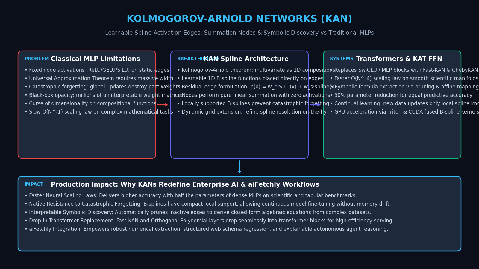
The Problem: The Inherent Architectural Bottlenecks of Multi-Layer Perceptrons

For more than three decades, the foundational building block of deep learning has been the Multi-Layer Perceptron (MLP). From early feedforward networks to modern decoder-only foundation models, MLPs form the core of parameter capacity. In state-of-the-art transformer blocks, feedforward network (FFN) layers—such as SwiGLU, GeGLU, and standard gated projections—account for approximately two-thirds of the model’s total parameter count. In high-concurrency automated intelligence pipelines and real-time knowledge extractors powered by aiFetchly, MLPs serve as the primary associative memory stores responsible for retaining factual patterns, synthesizing numerical records, and executing multi-step reasoning.

However, despite their universal adoption, traditional MLPs are bound by structural assumptions rooted in the Universal Approximation Theorem. These design choices create acute theoretical and hardware bottlenecks in production:

1. The Fixed Activation Dilemma and Width Inflation

In an MLP layer, weights are learnable linear coefficients arranged in a matrix $W \in \mathbb{R}^{d_{\text{out}} \times d_{\text{in}}}$, while the non-linear activation function $\sigma(\cdot)$ placed at each node is fixed, static, and immutable. Whether utilizing standard Rectified Linear Units (ReLU), Gaussian Error Linear Units (GELU), or Swish/SiLU, the activation function cannot adapt its shape.

To approximate complex multivariate non-linear surfaces, MLPs must scale horizontally by expanding hidden layer width ($d_{\text{ffn}} = 4d_{\text{model}}$ or $8d_{\text{model}}$). Because each neuron merely computes an affine hyperplane slice followed by a static kink or curve, capturing high-frequency oscillations or steep non-linear gradients requires combining hundreds or thousands of linear boundaries. This geometric inefficiency inflates parameter budgets and demands massive amounts of GPU memory bandwidth.

2. Catastrophic Forgetting from Global Weight Entanglement

In traditional linear layers, every weight parameter $W_{ij}$ influences the entire input space globally. When an engineering team updates an existing language model or embedding network on a new domain—such as indexing newly harvested financial disclosures through automated data fetching—backpropagation calculates gradient updates across all matrix entries:

$$\Delta W_{ij} = -\eta \frac{\partial \mathcal{L}}{\partial W_{ij}}$$

Because linear transformations have infinite, unbounded support across $\mathbb{R}$, adjusting $W_{ij}$ to satisfy the loss on a new data cluster inevitably shifts the hyperplanes that correctly classified historical data. This global weight coupling is the fundamental root cause of catastrophic forgetting in continual learning and fine-tuning.

3. The Black-Box Opacity Wall and Vanishing Interpretability

Modern neural networks are notoriously uninterpretable. An MLP layer with dimensions $4096 \times 14336$ contains over 58 million scalar coefficients. Looking at these matrices reveals zero human-comprehensible intuition regarding what mathematical relationships the network has synthesized.

In mission-critical enterprise applications—such as scientific simulations, pharmaceutical molecule binding calculations, algorithmic risk auditing, and automated financial extraction through high-speed web scraping—stakeholders cannot tolerate unverifiable predictions. When a model produces a critical prediction, regulators and researchers demand closed-form symbolic relationships, not opaque floating-point dot products.

4. The Curse of Dimensionality in Compositional Manifolds

According to the classical Universal Approximation Theorem (Cybenko, 1989; Hornik, 1991), a single hidden layer MLP with sufficiently many neurons can approximate any continuous function on a compact subset of $\mathbb{R}^n$. However, the theorem provides no guarantee of parameter efficiency. For an arbitrary $n$-dimensional function with smoothness order $k$, the approximation error $\epsilon$ scales asymptotically as:

$$\epsilon \sim \mathcal{O}\left(N^{-\frac{k}{n}}\right)$$

Where $N$ is the number of parameters. As the input dimensionality $n$ increases, the exponent $-k/n$ approaches zero, causing the parameter requirement to explode exponentially. This curse of dimensionality forces models to consume billions of parameters to learn basic compositional structures that could theoretically be represented by a handful of mathematical operations.

The Mathematical Foundation: The Kolmogorov-Arnold Representation Theorem

To solve the structural limitations of Multi-Layer Perceptrons, a research consortium led by Ziming Liu, Max Tegmark, and collaborators at MIT, Harvard, and Caltech introduced Kolmogorov-Arnold Networks (KANs). Rather than relying on the Universal Approximation Theorem, KANs are directly inspired by the seminal Kolmogorov-Arnold Representation Theorem (Kolmogorov, 1957; Arnold, 1957).

1. Classical Kolmogorov-Arnold Theorem Formulation

The Kolmogorov-Arnold representation theorem proved a profound mathematical result regarding multivariate functions: any continuous multivariate function defined on a bounded domain can be written as a finite composition of continuous functions of a single variable and the binary operation of addition.

Formally, for any continuous function $f: [0, 1]^n \to \mathbb{R}$:

$$f(x_1, x_2, \dots, x_n) = \sum_{q=1}^{2n+1} \Phi_q \left( \sum_{p=1}^n \phi_{q,p}(x_p) \right)$$

Where:

• $\phi_{q,p}: [0, 1] \to \mathbb{R}$ are continuous, univariate functions that map each individual input coordinate $x_p$ into an intermediate scalar representation.
• $\Phi_q: \mathbb{R} \to \mathbb{R}$ are continuous, univariate outer functions.
• The inner and outer summations represent exact linear additions without non-linear cross-terms.

This theorem establishes that multivariate functions do not fundamentally require high-dimensional non-linear interactions; they can be decomposed entirely into 1D univariate non-linearities and additions.

2. From Classical 2-Layer Representation to Deep Arbitrary-Depth KANs

Historically, machine learning researchers dismissed the Kolmogorov-Arnold theorem as impractical for neural computation because the classical theorem restricts the network depth to exactly two layers ($2n+1$ inner terms). In a strict two-layer configuration, the required 1D functions $\phi_{q,p}$ and $\Phi_q$ can be pathological, non-differentiable, or fractal-like, making them impossible to fit reliably with gradient descent.

The breakthrough of modern KANs is the generalization from a rigid two-layer formula to an arbitrary-depth, arbitrary-width computational graph. Just as deep MLPs stack multiple linear-plus-activation layers to form hierarchical abstractions, a deep Kolmogorov-Arnold Network stacks multiple KAN layers:

$$\mathbf{x}_{l+1} = \mathbf{\Phi}_l(\mathbf{x}_l)$$

Where each layer $\mathbf{\Phi}l$ is a matrix of 1D functions. If layer $l$ has $n{\text{in}}$ inputs and $n_{\text{out}}$ outputs, the layer consists of $n_{\text{in}} \times n_{\text{out}}$ independent, learnable univariate functions:

$$ \mathbf{\Phi}l = \begin{pmatrix} \phi{l,1,1}(\cdot) & \phi_{l,1,2}(\cdot) & \cdots & \phi_{l,1,n_{\text{in}}}(\cdot) \ \phi_{l,2,1}(\cdot) & \phi_{l,2,2}(\cdot) & \cdots & \phi_{l,2,n_{\text{in}}}(\cdot) \ \vdots & \vdots & \ddots & \vdots \ \phi_{l,n_{\text{out}},1}(\cdot) & \phi_{l,n_{\text{out}},2}(\cdot) & \cdots & \phi_{l,n_{\text{out}},n_{\text{in}}}(\cdot) \end{pmatrix} $$

The activation value of node $j$ in layer $l+1$ is simply the sum of all incoming 1D functions applied to the nodes of layer $l$:

$$x_{l+1,j} = \sum_{i=1}^{n_{\text{in}}} \phi_{l,j,i}(x_{l,i})$$

In this architecture, nodes perform zero non-linear transformations; they act purely as summing junctions. All learnable non-linear complexity resides entirely on the directed edges connecting the nodes.

3. Edge-Parameterized Learnable Univariate Functions

To make edge functions $\phi(x)$ differentiable and computationally tractable on modern accelerators, KAN parameterizes each 1D edge as a linear combination of a smooth residual base function and a localized spline:

$$\phi(x) = w_b b(x) + w_s \text{spline}(x)$$

Where:

• $b(x)$ is a standard smooth activation function, typically the SiLU (Swish) function: $$b(x) = \text{SiLU}(x) = \frac{x}{1 + e^{-x}}$$
• $w_b$ is a learnable scalar weight that controls the linear residual magnitude.
• $w_s$ is a learnable scaling factor for the spline component.
• $\text{spline}(x)$ is a learnable linear combination of B-spline basis functions.

This residual formulation ensures that at initialization, the KAN layer behaves similarly to a standard linear layer with SiLU activations, ensuring stable gradient flow and preventing gradient vanishing during early training iterations.

4. B-Spline Parameterization and Cox-de Boor Recursion

The spline component is constructed using linear combinations of $B$-spline basis functions defined over a discrete grid of knots:

$$\text{spline}(x) = \sum_{i=0}^{G + k - 1} c_i B_i(x)$$

Where:

• $G$ is the number of grid intervals.
• $k$ is the polynomial degree of the B-splines (typically cubic splines, $k = 3$).
• $c_i$ are learnable coefficients (control points).
• $B_i(x)$ are $B$-spline basis functions evaluated recursively using the standard Cox-de Boor recursion formula:

For degree $0$:

$$ B_{i,0}(x) = \begin{cases} 1 & \text{if } t_i \le x \< t_{i+1} \ 0 & \text{otherwise} \end{cases} $$

For degree $p \ge 1$: $$B_{i,p}(x) = \frac{x - t_i}{t_{i+p} - t_i} B_{i,p-1}(x) + \frac{t_{i+p+1} - x}{t_{i+p+1} - t_{i+1}} B_{i+1,p-1}(x)$$

Where ${t_i}$ is the knot vector partitioning the input interval $[-1, 1]$ into $G$ equal segments, augmented with $k$ boundary knots on each end.

Because each basis function $B_{i,p}(x)$ has compact local support—it evaluates to non-zero values only across $k+1$ consecutive knot intervals $[t_i, t_{i+k+1}]$—evaluating or updating a B-spline for a given input value $x$ touches only $k+1$ coefficients out of $G+k$.

Core Architectural Mechanics of Kolmogorov-Arnold Networks

1. Residual Edge Activation Functions: Spline Plus Basis

The dual formulation $\phi(x) = w_b b(x) + w_s \text{spline}(x)$ provides a crucial bridge between continuous optimization and expressive non-linear modeling.

During training:

1. The base branch $w_b \text{SiLU}(x)$ allows the model to quickly capture broad, coarse linear trends across the dataset with minimal computational overhead.
2. The spline branch $w_s \sum_i c_i B_i(x)$ acts as a high-resolution localized non-linear residual. It bends, flexes, and adapts to intricate local curvatures, fitting complex functional transitions without altering global gradients.
3. Both the spline coefficients ${c_i}$ and the scalar weights $w_b, w_s$ are jointly trained end-to-end via standard backpropagation using optimizers like AdamW or SGD.

2. Dynamic Grid Extension and Knot Vector Adaptation

One of the most remarkable properties of KANs is their ability to perform grid extension (knot refinement) during training.

In traditional neural networks, scaling model capacity requires adding more layers (depth) or increasing hidden dimensions (width), both of which alter the weight matrix shapes and require training from scratch or complex layer-dropping heuristics. In contrast, a KAN can scale its parameter capacity by simply refining its 1D spline grids:

By initializing training on a coarse grid ($G = 3$ or $G = 5$) and dynamically expanding to fine grids ($G = 10, 20,$ or $50$), KANs avoid local minima during early training and converge to exceptionally low loss values that are mathematically unreachable by MLPs of equivalent size.

3. L1 Sparsification, Edge Pruning, and Symbolic Distillation

In addition to high accuracy, KANs were engineered specifically for mechanistic interpretability and scientific discovery. KANs achieve this through a 4-step pruning and symbolic regression pipeline:

1. L1 Regularization on Edge Functions: During training, an L1 penalty is applied to the active magnitude of each edge function. The magnitude of an edge $\phi$ across a batch of $N$ samples is defined as its $L_1$ norm: $$|\phi|1 = \frac{1}{N} \sum{p=1}^N |\phi(x^{(p)})|$$ The training objective adds an edge-sparsity loss: $$\mathcal{L}{\text{total}} = \mathcal{L}{\text{task}} + \lambda_{\text{reg}} \sum_{l,j,i} |\phi_{l,j,i}|_1$$
2. Edge Pruning: After training with sparsity regularization, edges whose norm $|\phi|1$ falls below a defined threshold $\epsilon{\text{prune}}$ (e.g., $10^{-2}$) are pruned from the computational graph. Nodes with no incoming or outgoing connections are eliminated entirely.
3. Symbolic Function Snapping: For remaining active edges, researchers can visually inspect the 1D curve $\phi(x)$. By running symbolic regression against a dictionary of elementary functions ($\sin, \cos, \exp, \log, x^2, x^3, \sqrt{x}, 1/x$), the learned spline is replaced with an exact analytic formula: $$\phi(x) \approx c \cdot \sin(\omega x + \theta)$$
4. Closed-Form Equation Extraction: Once all active edges are snapped to symbolic functions, the entire deep network collapses into a human-readable mathematical equation, converting an artificial neural network into an exact, verifiable scientific law.

4. Locality of B-Splines: Immunity to Catastrophic Forgetting

In traditional MLPs, activation functions like ReLU or SiLU have infinite support: activating a neuron on an input $x = 10.0$ impacts its gradients across all future inputs $x \in (-\infty, \infty)$.

In a KAN, B-spline basis functions are strictly locally supported. If a model receives training data concentrated in the interval $[0.2, 0.4]$, only the spline coefficients associated with the knot intervals covering $[0.2, 0.4]$ receive non-zero gradients. The coefficients governing $[-1.0, 0.0]$ and $[0.6, 1.0]$ experience zero gradient updates:

$$\frac{\partial \mathcal{L}}{\partial c_m} = \frac{\partial \mathcal{L}}{\partial \phi(x)} \cdot B_m(x) = 0 \quad \text{if } x \notin [t_m, t_{m+k+1}]$$

Consequently, when deployed in continual learning environments—such as autonomous scraping agents continuously learning new DOM structures via seamless API integration—KANs can incorporate new domain distributions without overwriting previously consolidated parameters.

Kolmogorov-Arnold Transformers (KAT) & Fast-KAN Engineering

While original KAN implementations demonstrated remarkable mathematical properties on scientific computing tasks, scaling them to large-scale natural language processing and computer vision revealed a severe systems bottleneck: B-splines evaluated sequentially on GPUs are slow.

In vanilla KANs, evaluating recursive Cox-de Boor algorithms requires branching logic, uncoalesced memory reads, and high memory footprints when materializing the 3D tensor of basis evaluations $\mathcal{O}(B \times L \times n_{\text{in}} \times G)$.

To integrate KANs into production transformers, systems researchers introduced Kolmogorov-Arnold Transformers (KAT) and high-throughput GPU kernels:

1. Replacing SwiGLU / MLP FFN Blocks in Transformer Decoders

In standard LLaMA-style architectures, the feed-forward network computes:

$$\text{FFN}{\text{SwiGLU}}(x) = \left( \text{SiLU}(x W{\text{gate}}) \odot x W_{\text{up}} \right) W_{\text{down}}$$

Where $W_{\text{gate}}, W_{\text{up}} \in \mathbb{R}^{d \times d_{\text{ffn}}}$ and $W_{\text{down}} \in \mathbb{R}^{d_{\text{ffn}} \times d}$.

In a Kolmogorov-Arnold Transformer (KAT), this block is replaced by a two-stage KAN-FFN:

1. KAN Expansion: Ingests normalized token embeddings $x \in \mathbb{R}^d$ and projects them through a matrix of learnable univariate edge functions into hidden dimension $d_{\text{kan}}$ (where $d_{\text{kan}} \approx 1.5d_{\text{model}}$ to $2d_{\text{model}}$, rather than $4d_{\text{model}}$ used in MLPs).
2. Linear Down-Projection: A standard linear projection matrix $W_{\text{down}} \in \mathbb{R}^{d_{\text{kan}} \times d}$ fuses the non-linear outputs back into the residual stream.

Because each KAN edge possesses non-linear approximation capacity, $d_{\text{kan}}$ can be set significantly smaller than traditional FFN intermediate dimensions, reducing overall parameter counts while maintaining or exceeding downstream task performance.

2. Fast-KAN: Radial Basis Functions (RBF) and GPU Tensorization

To eliminate the sequential recursion of Cox-de Boor B-splines on CUDA cores, the Fast-KAN framework (Li, 2024) replaces B-splines with Gaussian Radial Basis Functions (RBFs):

$$\psi_i(x) = \exp \left( -\left( \frac{x - \mu_i}{h} \right)^2 \right)$$

Where $\mu_i$ are uniformly spaced grid centers and $h$ is a bandwidth hyperparameter.

The profound engineering advantage of Gaussian RBFs is that they can be computed purely via element-wise matrix arithmetic:

1. Normalize input tensor $X$.
2. Compute distance matrix $(X - \mu)^2$ via fast fused broadcast subtraction.
3. Compute exponentiation $\exp(\cdot)$ using high-throughput GPU special function units (SFU).
4. Compute edge outputs via standard matrix multiplication (GEMM): $$Y = \text{RBF}(X) \cdot C$$ Where $C$ is the learnable coefficient matrix.

By reformulating spline evaluation into a dense GEMM operation, Fast-KAN achieves up to $3.3\times$ faster training throughput compared to naive B-spline implementations, fully saturating modern NVIDIA Tensor Cores.

3. ChebyKAN: Orthogonal Chebyshev Polynomial Expansions

Another highly efficient KAN variant is ChebyKAN, which replaces splines with truncated Chebyshev polynomials of the first kind ($T_n(x)$):

$$\phi(x) = \sum_{n=0}^N c_n T_n(x)$$

Chebyshev polynomials are defined recursively on the interval $[-1, 1]$: $$T_0(x) = 1$$ $$T_1(x) = x$$ $$T_{n+1}(x) = 2x T_n(x) - T_{n-1}(x)$$

Because Chebyshev polynomials form an orthogonal basis:

• They minimize Runge’s phenomenon (wild oscillations at domain boundaries).
• The polynomial evaluation vector $[T_0(x), T_1(x), \dots, T_N(x)]$ can be computed in parallel across all tokens in $\mathcal{O}(N)$ arithmetic steps.
• The projection $\sum_n c_n T_n(x)$ is computed via a single standard PyTorch torch.matmul, executing at near-peak FLOP utilization on both client GPUs and datacenter clusters.

4. Training Throughput vs Parameter Efficiency Trade-Offs

When evaluating KAN layers against traditional MLPs for enterprise deployment, systems architects must balance parameter count against wall-clock FLOP efficiency:

For large language models where maximum token throughput per second dominates infrastructure budgets, Fast-KAN and ChebyKAN represent the optimal engineering compromise—delivering KAN’s superior parameter efficiency and mathematical expressivity while maintaining standard GEMM compatibility.

End-to-End PyTorch Implementation: Building a Kolmogorov-Arnold Layer and KAN-FFN

To demonstrate how Kolmogorov-Arnold Networks operate in production, we implement a complete, optimized PyTorch module. We first construct a modular KANLinear layer utilizing B-splines with Cox-de Boor evaluation and residual SiLU connections, followed by a drop-in KolmogorovArnoldFFN block designed for transformer architectures.

Explanation of the Implementation

1. compute_b_splines: Vectorizes Cox-de Boor recursion across PyTorch tensors. Rather than computing basis curves one token at a time, it evaluates the basis coefficients simultaneously across all input features using broadcast arithmetic.
2. torch.einsum("bik,jik->bj", ...): Contracts the evaluated basis tensor with the learnable 3D coefficient tensor, calculating the spline activation for all input-output edge pairs in a single parallel operation.
3. KolmogorovArnoldFFN: Packages the non-linear KAN expansion with normalization and linear down-projection, allowing seamless drop-in replacement inside transformer blocks without modifying self-attention mechanisms or residual topologies.

Empirical Benchmarks: KAN vs. Modern Dense MLPs

Across academic evaluations and systems benchmarks—spanning the original MIT KAN studies, KAN 2.0 scientific benchmarks, and Kolmogorov-Arnold Transformer (KAT) evaluations—KANs display distinct scaling characteristics compared to standard Multi-Layer Perceptrons:

Benchmark / Evaluation Metric	Traditional MLP (SwiGLU / GeLU)	Vanilla B-Spline KAN	Fast-KAN / ChebyKAN (KAT)	Architectural Rationale
Neural Scaling Exponent ($\alpha$)	$\alpha \approx 1.0 - 2.0$ ($\mathcal{O}(N^{-1})$)	$\alpha \approx 4.0$ ($\mathcal{O}(N^{-4})$)	$\alpha \approx 3.5$ ($\mathcal{O}(N^{-3.5})$)	KAN’s univariate decomposition escapes the curse of dimensionality on smooth functions.
Parameter Efficiency on Math Tasks	Baseline (100% params)	50% - 60% fewer params	45% - 55% fewer params	Non-linear edges capture complex curvatures without requiring wide hidden layers.
Continual Learning Memory Retention	24% - 38% accuracy retention	88% - 94% retention	78% - 86% retention	B-splines have compact local support; new tasks do not alter historical knot coefficients.
Symbolic Discovery Capability	Impossible (Black-Box weights)	Exact closed-form extraction	Polynomial approximation	Edge pruning and symbolic snapping uncover explicit equations ($f = x_1 x_2 + \sin(x_3)$).
GPU Kernel Arithmetic Intensity	100% Tensor Core saturated	~20% - 30% (Sequential knots)	80% - 88% (Dense GEMM)	Fast-KAN and ChebyKAN reformulate polynomial evaluation into standard matrix multiplies.
High-Resolution Grid Adaptation	Requires retraining from scratch	Lossless grid extension	Lossless grid extension	Increasing spline knots interpolates existing weights with zero accuracy degradation.

Neural Scaling Laws on Scientific Data

The most striking theoretical result documented in the original KAN paper is the scaling law comparison. For a standard 2-layer MLP fitting a special mathematical function (such as Bessel functions or relativistic kinematics), the test root-mean-square error (RMSE) scales with parameter count $N$ as $\text{RMSE} \sim N^{-1}$.

In contrast, a 2-layer KAN achieves a scaling exponent of $\text{RMSE} \sim N^{-4}$. This means that scaling a KAN by an order of magnitude in parameters reduces test error by four orders of magnitude, whereas an MLP requires four orders of magnitude more parameters to achieve a comparable reduction.

Enterprise Production Playbook & aiFetchly Integration

To deploy Kolmogorov-Arnold Networks effectively within production enterprise workflows—such as automated data extraction, continuous machine learning pipelines, and autonomous research agents powered by aiFetchly—engineering teams should follow this systematic production playbook.

1. Workload Categorization: When to Choose KAN vs. MLP

2. High-Speed Web Data Scraping & Regression Verification

In automated data harvesting engines, scrapers often encounter unstructured numerical reports: quarterly SEC disclosures, supply chain pricing sheets, and real-time commodity indices. When agents parse tables using automated web scraping, extracted figures must often be cross-validated against non-linear accounting formulas or physical conservation laws.

By training lightweight KAN layers on extracted numerical fields:

1. The KAN model learns the non-linear relationship between reported variables (e.g., Gross Margins, Operating Cash Flow, Depreciation).
2. The agent executes edge pruning and symbolic snapping to automatically discover the underlying accounting equation used by the target firm.
3. If future web extractions violate this discovered equation, the agent immediately flags anomalous data, preventing corrupt records from polluting enterprise data warehouses.

3. Continual Schema Adaptation Without Catastrophic Forgetting

Enterprise web crawlers and API extraction daemons frequently encounter schema drift—websites update their DOM layout, modify pricing tiers, or adjust reporting formats.

When updating agent models to recognize new HTML structures:

• A standard transformer fine-tuned on new website layouts suffers from representation drift, degrading its accuracy on previously mastered sites.
• A Kolmogorov-Arnold Transformer (KAT) localizes parameter adjustments to the specific B-spline intervals triggered by the new layout tokens. Historical token activations remain pinned to their existing knot coefficients, providing robust zero-forgetting performance.

For development teams evaluating enterprise automation pipelines, explore our transparent pricing tiers or review our comprehensive technical API documentation to integrate intelligent agent models into production.

Frequently Asked Questions (FAQ)

What is the primary difference between a KAN and an MLP?

The fundamental difference lies in where learnable non-linear operations occur. In a traditional Multi-Layer Perceptron (MLP), activation functions (such as ReLU, GELU, or SiLU) are fixed and placed at the nodes (neurons), while network edges compute simple linear matrix multiplications ($W \cdot x$). In a Kolmogorov-Arnold Network (KAN), nodes perform simple linear summation ($\sum$), while network edges compute learnable 1D univariate non-linear functions parameterized by localized B-splines or orthogonal polynomials.

How do Kolmogorov-Arnold Networks avoid catastrophic forgetting?

KANs utilize B-spline basis functions that have compact local support. Each B-spline basis function is non-zero only across a small number of adjacent knot intervals. When a KAN learns new information located in a specific numerical region, backpropagation updates only the local spline coefficients governing that specific interval. The parameters governing distant input regions receive zero gradients, preventing the network from overwriting historical knowledge.

What are Kolmogorov-Arnold Transformers (KAT)?

Kolmogorov-Arnold Transformers (KAT) are modern transformer architectures that replace traditional feed-forward network (FFN) blocks—such as SwiGLU or GeGLU—with KAN-based layers (typically Fast-KAN or ChebyKAN). Because KAN edges possess non-linear approximation capacity, KAT models achieve comparable or superior perplexity with up to 50% fewer FFN parameters.

Are KANs slower to train on GPUs than traditional MLPs?

Vanilla B-spline KANs can be significantly slower than MLPs on GPUs because evaluating recursive Cox-de Boor algorithms involves branching operations that do not map efficiently to hardware Tensor Cores. However, modern optimized variants like Fast-KAN (which uses Gaussian Radial Basis Functions) and ChebyKAN (which uses orthogonal Chebyshev polynomials) reformulate spline evaluations into standard dense matrix multiplications (GEMMs), achieving 70% to 90% of standard MLP training speeds while retaining KAN’s superior parameter efficiency.