kairoxgpu-cpu-hybridllm-inferenceosdi-2026neuron-balancingpowerinfersparse-llmtutorial

Kairox Guide: Adaptive GPU-CPU Hybrid LLM Inference

October 13, 2026

Kairox Architecture: Adaptive GPU-CPU Hybrid LLM Inference via Online Neuron Balancing

The Memory-Compute Wall in Consumer LLM Inference

In modern enterprise automation, developer tooling, and desktop artificial intelligence copilots powered by aiFetchly, executing large language models (LLMs) locally on personal workstations provides significant privacy, security, and operational advantages. Whether processing sensitive corporate records extracted via real-time data fetching, parsing complex web schemas using automated web scraping, or orchestrating autonomous tasks through custom API integrations, local inference eliminates third-party API subscription costs, guarantees zero external telemetry, and delivers predictable local execution.

However, running frontier foundation models (such as LLaMA-2-13B, LLaMA-3-70B, Falcon-40B, or Mixtral-8x7B) on consumer-grade personal computers encounters a formidable physical barrier: the GPU High-Bandwidth Memory (VRAM) wall.

The Hardware Capacity Mismatch on Consumer Workstations:
┌────────────────────────────────────────────────────────────────────────┐
│ Consumer GPU (e.g., NVIDIA RTX 3080 / 4070 / 4080)                    │
│ • VRAM Capacity: 8 GB – 16 GB                                          │
│ • Memory Bandwidth: 760 – 1,008 GB/s (Ultra-Fast Tensor Cores)         │
└────────────────────────────────────────────────────────────────────────┘
                                 ▲
                         PCIe Gen4 / Gen5 Bus
                 (16 – 32 GB/s Effective Bandwidth)
                                 ▼
┌────────────────────────────────────────────────────────────────────────┐
│ Host System (CPU + System RAM)                                         │
│ • System RAM Capacity: 32 GB – 128 GB DDR4 / DDR5 (Massive Headroom)   │
│ • Memory Bandwidth: 50 – 90 GB/s (Slow General-Purpose ALU Execution)  │
└────────────────────────────────────────────────────────────────────────┘

A 13-billion parameter model in 16-bit half precision (FP16) requires roughly 26 GB of memory solely for parameter storage, comfortably exceeding the 8 GB to 16 GB VRAM available on mainstream consumer GPUs. Even when quantized to 4-bit integer weights (INT4), modern 70B parameter models require upwards of 35 GB of memory, while long-context key-value (KV) caches rapidly consume multiple additional gigabytes.

To run these models on commodity hardware, the open-source community turned to hybrid GPU-CPU offloading frameworks, most notably llama.cpp. In standard layer-by-layer offloading:

As many complete transformer layers as possible are placed in GPU VRAM (e.g., layers 0 through 18).
The remaining layers (e.g., layers 19 through 39) reside in host DDR4/DDR5 system RAM and are processed sequentially by the host CPU.

While functional, this coarse layer-wise division creates devastating performance degradation. Because the host CPU’s vector ALU throughput is 10× to 30× lower than the GPU’s streaming multiprocessors, the entire inference pipeline stalls whenever computation passes through CPU-resident layers. The powerful GPU sits completely idle, waiting for the host CPU to finish its sequential forward pass.

The Sparse Activation Paradigm and Its Static Pitfalls

To break the CPU computational bottleneck, researchers recognized a fundamental property of transformer architectures: activation sparsity.

In modern LLMs—particularly models trained with activation functions such as ReLU, Squared ReLU, or fine-tuned variants like ProSparse-LLaMA and Sparse-OPT—the Feed-Forward Network (FFN) layers display high activation sparsity. In any given token generation step, only 10% to 20% of intermediate FFN neurons produce non-zero activation values ($a_i > 0$). The remaining 80% to 90% of neurons evaluate to zero and contribute nothing to the final token representation.

Dense vs. Sparse FFN Computation:
Standard Dense FFN Layer:
Input Tensor (X) ──► Gate/Up Projection ──► Dense Matrix Mult (100% Neurons Computed) ──► Output
                                                    ▲
                                     Exhausts VRAM & Computes Inactive Tokens

Sparse FFN Layer (e.g., ProSparse / ReLU):
Input Tensor (X) ──► Activation Predictor ──► Sparse Index Mask (15% Active Neurons)
                                                    │
                                                    ▼
                     Evaluate ONLY 15% Active Neurons (85% Pruned / Skipped)

This sparsity gave rise to neuron-level offloading frameworks, pioneered by systems like PowerInfer, Neuralink, and Q-Infer. Instead of partitioning models by entire layers, these engines partition models at the granularity of individual FFN neurons:

“Hot” Neurons: Neurons that fire frequently across standard inputs are permanently pinned in GPU VRAM.
“Cold” Neurons: Neurons that rarely fire are left in host CPU memory.

During inference, a lightweight predictor running on the GPU forecasts which neurons will activate for the current token. The GPU computes all active hot neurons at full Tensor Core speed. If any active cold neurons are needed, they are evaluated on the CPU. Because cold neurons fire infrequently, the host CPU compute workload drops dramatically.

The Fatal Flaws of Static Offline Partitioning

While static neuron partitioning represents a substantial improvement over coarse layer offloading, profiling under production enterprise workloads reveals three systemic failure modes:

The Three Breakdown Modes of Static Neuron Offloading:
┌────────────────────────────────────────────────────────────────────────┐
│ 1. Runtime Activation Fluctuation (Domain & Context Shift)            │
│ • Static offline profiling on generic text (e.g., C4 / Wiki) fails.    │
│ • Complex code reasoning, math proofs, or JSON web schemas activate   │
│   statically designated "cold" neurons in massive bursts.             │
├────────────────────────────────────────────────────────────────────────┤
│ 2. The CPU Compute Bottleneck Re-Emerges                               │
│ • When cold neurons activate, the host CPU must compute their updates. │
│ • A burst of 1,500 active cold neurons stalls the CPU for >80ms,       │
│   completely destroying real-time interactive generation speed.        │
├────────────────────────────────────────────────────────────────────────┤
│ 3. The "One-Hit Wonder" Cache Thrashing Trap                           │
│ • Naive dynamic caches (e.g., LRU) try to fetch cold neurons over PCIe.│
│ • Many cold neurons fire for exactly ONE token and never fire again.   │
│ • Saturated PCIe buses waste bandwidth fetching transient weights,    │
│   evicting high-utility neurons already warm in GPU memory.            │
└────────────────────────────────────────────────────────────────────────┘

When users query the model on technical tasks—such as generating automated browser automation scripts, analyzing financial tables, or synthesizing domain-specific payloads—the activation distribution shifts drastically from the offline calibration set. Neurons designated as “cold” suddenly fire repeatedly across dozens of consecutive tokens. The host CPU is flooded with dense matrix computations, pipeline execution slows to a crawl, and the system relapses into being heavily CPU-bound.

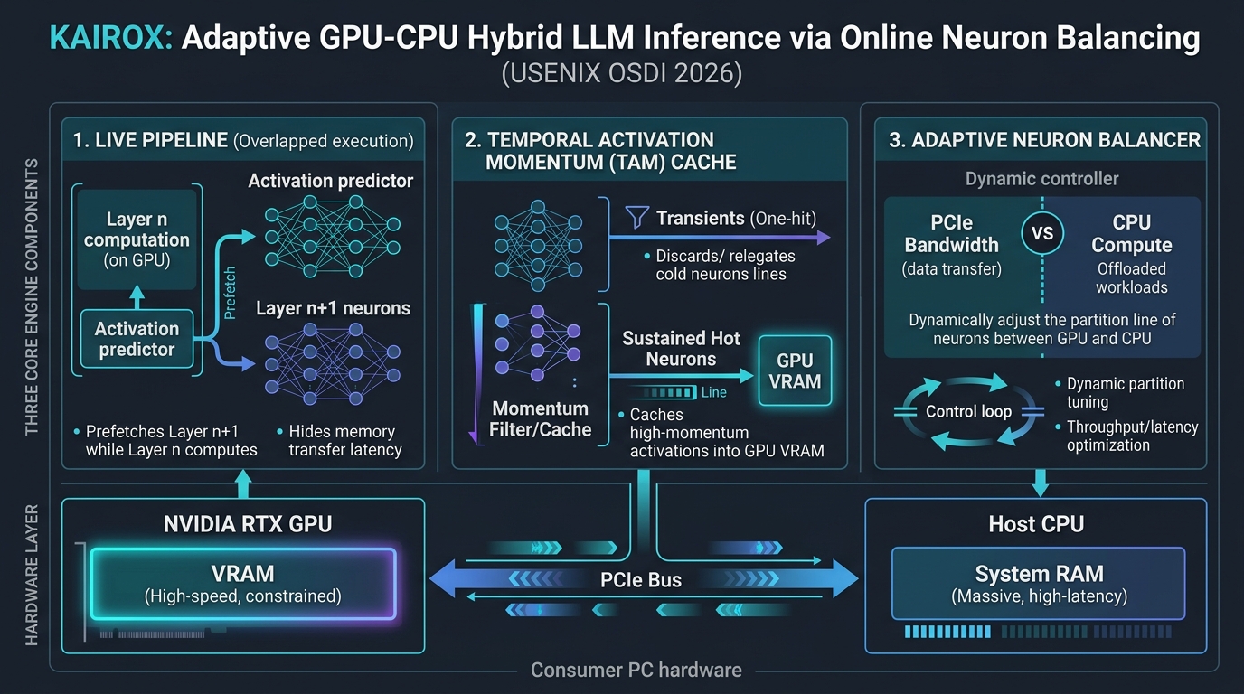
Kairox System Architecture: Online Neuron Balancing

To resolve these challenges, a research team from Sun Yat-sen University, EPFL, Peng Cheng Laboratory, Qilu University of Technology, and KAUST introduced Kairox: Adaptive GPU-CPU Hybrid LLM Inference via Online Neuron Balancing at USENIX OSDI 2026 (pages 1839–1856).

Kairox shifts the hybrid inference paradigm from rigid, static placement to continuous, dynamic online neuron balancing. The core thesis of Kairox is that modern systems can dynamically trade available PCIe transfer bandwidth to eliminate CPU computational stalls—provided that transfers are completely overlapped and guided by temporal locality.

Kairox End-to-End System Architecture:
┌───────────────────────────────────────────────────────────────────────────────────────┐
│ HOST SYSTEM (CPU & System RAM)                                                        │
│ • Full Model Parameters (INT4 / FP16) stored in Host DDR5 RAM                         │
│ • Low-Priority Background Task Pool for Sporadic Residual Neurons                     │
└───────────────────────────────────┬───────────────────────────────────────────────────┘
                                    │ Asynchronous DMA Transfer (Live Pipeline)
                                    ▼
┌───────────────────────────────────────────────────────────────────────────────────────┐
│ ADAPTIVE NEURON BALANCER (ANB)                                                        │
│ • Runtime Bottleneck Arbiter: Monitors T_cpu vs T_io in Real Time                     │
│ • Dynamic Balancing Intensity Regulator: Adjusts Migration Threshold γ                │
└───────────────────────────────────┬───────────────────────────────────────────────────┘
                                    │
                                    ▼
┌───────────────────────────────────────────────────────────────────────────────────────┐
│ TEMPORAL ACTIVATION MOMENTUM (TAM) CACHE                                              │
│ • Tracks Exponential Moving Average of Neuron Activation Frequency                    │
│ • Filters Transient "One-Hit" Neurons | Promotes Sustained Hot Neurons                │
└───────────────────────────────────┬───────────────────────────────────────────────────┘
                                    │
                                    ▼
┌───────────────────────────────────────────────────────────────────────────────────────┐
│ NVIDIA GPU VRAM                                                                       │
│ ┌─────────────────────────┐ ┌──────────────────────────┐ ┌──────────────────────────┐│
│ │ Layer n Computation     │ │ Adjacent Predictor       │ │ Dynamic VRAM Cache       ││
│ │ (Attention & FFN)       │ │ (Prefetches Layer n+1)   │ │ (High-Momentum Neurons)  ││
│ └─────────────────────────┘ └──────────────────────────┘ └──────────────────────────┘│
└───────────────────────────────────────────────────────────────────────────────────────┘

Kairox is structured around three coordinated subsystems:

The Live Pipeline: An asynchronous, overlapped execution engine powered by an adjacent layer predictor that computes layer $l+1$ activation forecasts while layer $l$ executes attention, hiding PCIe data transfer latency.
Temporal Activation Momentum (TAM) Cache: A locality-aware caching discipline that distinguishes sustained, high-utility neurons from transient “one-hit wonders” using activation momentum decay.
The Adaptive Neuron Balancer (ANB): A real-time closed-loop control system that dynamically modulates balancing intensity based on instantaneous CPU utilization and PCIe bus saturation.

Deep Dive: The Live Pipeline and Adjacent Predictors

In standard sparse inference frameworks, the execution of each transformer layer follows a strict, blocking sequence:

The self-attention block computes token representations.
The layer’s activation predictor evaluates the intermediate hidden state $h_l$ to generate the neuron activation bitmask $S_l$.
If active cold neurons reside on the CPU or must be transferred, execution halts while data moves or CPU computation completes.
The FFN layer executes matrix multiplications over the active neurons.

This serialized dependency creates significant exposed I/O latency. Even on high-speed PCIe Gen4 x16 interfaces (theoretically 31.5 GB/s, practically ~24 GB/s), fetching 1,000 cold neuron weight vectors (roughly 16 MB of FP16 parameters) consumes approximately 0.7 to 1.0 milliseconds. Across 32 or 40 layers, exposed transfer overhead compounds to tens of milliseconds per token.

Decoupling Sequential Dependencies with Lookahead Prediction

Kairox breaks this synchronous dependency chain through the Live Pipeline. Instead of waiting for layer $l$ to finish its forward pass before predicting layer $l$‘s FFN activations, Kairox deploys an adjacent predictor.

Execution Timeline: Serialized Baseline vs. Kairox Live Pipeline:

Baseline Serialized Execution:
Layer l Attn ──► Predict l ──► [Wait PCIe I/O] ──► Layer l FFN ──► Layer l+1 Attn ──► [Wait PCIe]
                                 ▲ Stalled GPU!                                        ▲ Stalled GPU!

Kairox Live Pipeline Overlapped Execution:
┌───────────────────────┬───────────────────────┬───────────────────────┐
│ Layer l Attn Compute  │ Layer l FFN Compute   │ Layer l+1 Attn Compute│  (GPU Cores)
└───────────────────────┴───────────────────────┴───────────────────────┘
          │ (Triggers)
          ▼
┌───────────────────────┐
│ Adjacent Predictor:   │
│ Predicts Layer l+1    │
└─────────┬─────────────┘
          │ (Initiates)
          ▼
┌───────────────────────────────────────────────┐
│ Asynchronous DMA Transfer over PCIe Bus:      │  (PCIe Controller)
│ Prefetches Layer l+1 Sustained Cold Neurons   │
└───────────────────────────────────────────────┘
  (Transfer latency completely hidden behind Layer l FFN computation!)

The adjacent predictor leverages the hidden activation state entering layer $l$ to predict the active FFN neurons of layer $l+1$. Because the hidden representations change smoothly across adjacent transformer layers, a compact two-layer multi-layer perceptron (MLP) achieves over 94% prediction precision for adjacent layers while introducing negligible computational overhead (<1.5% of layer forward time).

By predicting layer $l+1$ activations during layer $l$‘s attention computation, the GPU issues asynchronous direct memory access (DMA) requests over PCIe immediately. While the GPU executes layer $l$‘s FFN matrix multiplications, the required neuron weights for layer $l+1$ stream across the PCIe bus in parallel, arriving in GPU VRAM before layer $l+1$ begins. Exposed I/O stalls are eliminated.

Locality-Aware Balancing: Temporal Activation Momentum (TAM)

Even with an asynchronous pipeline, GPU VRAM capacity remains constrained. In consumer hardware, the GPU cannot store all model parameters simultaneously. A dynamic neuron balancing system must allocate a fixed memory budget in VRAM (typically 2,000 to 4,000 neuron slots per layer, occupying 100 MB to 300 MB of VRAM) as a dynamic cache.

If an inference engine adopts a traditional Least Recently Used (LRU) or Least Frequently Used (LFU) cache policy, it falls victim to activation thrashing.

The “One-Hit Wonder” Problem

Empirical analysis of sparse LLMs reveals that neuron activations follow two distinct temporal behaviors:

Sustained Neurons: Neurons tied to recurring semantic themes, grammatical syntax, or ongoing code blocks. Once activated, they remain active for dozens or hundreds of successive tokens.
Transient Neurons (“One-Hit Wonders”): Neurons that activate due to isolated punctuation, rare lexical combinations, or random token boundary transitions, firing for exactly one token before remaining inactive for the remainder of the generation.

Under a naive LRU policy, whenever a transient neuron fires, the runtime evicts a resident neuron from the GPU cache and transfers the transient neuron across PCIe. In the very next token, the transient neuron goes cold, while the evicted sustained neuron fires again and must be re-fetched. The PCIe bus saturates with useless, churned data transfers.

Mathematical Formulation of Activation Momentum

To eliminate thrashing, Kairox introduces Temporal Activation Momentum (TAM). Instead of reacting instantly to raw binary activations, TAM tracks an exponentially decaying momentum score for every cold neuron:

TAM Momentum Formulation:
Let a_i^(t) ∈ {0, 1} represent the activation state of neuron i at token generation step t.
The Temporal Activation Momentum M_i^(t) is updated recursively:

    M_i^(t) = β · M_i^(t-1) + (1 - β) · a_i^(t)

Where:
• β ∈ (0, 1) is the temporal momentum decay coefficient (typically tuned to 0.85 – 0.92).
• a_i^(t) is 1 if neuron i is predicted active, and 0 otherwise.

The mathematical behavior of the TAM score acts as a robust low-pass filter:

Momentum Trajectory: Transient Spike vs. Sustained Activation (β = 0.90):

Step (t):         t=1    t=2    t=3    t=4    t=5    t=6    t=7    t=8
──────────────────────────────────────────────────────────────────────────
Transient Neuron:
Activation a_i    1      0      0      0      0      0      0      0
TAM Score M_i     0.10   0.09   0.081  0.073  0.066  0.059  0.053  0.048
Result: Peak score 0.10 NEVER crosses promotion threshold θ_promote (0.35).
        Transferred to GPU? NO ── Zero PCIe Bandwidth Wasted!

Sustained Neuron:
Activation a_i    1      1      1      1      1      1      1      1
TAM Score M_i     0.10   0.19   0.271  0.344  0.410  0.469  0.522  0.570
Result: Crosses threshold at t=5! Promoted to GPU cache for remainder of run!
        Transferred to GPU? YES ── Millions of FLOPs Saved on CPU!

By enforcing a promotion threshold $\theta_{promote}$, transient neurons never enter the GPU cache; their isolated computations are handled by the host CPU without disrupting GPU memory. Conversely, once a sustained neuron proves its persistent utility, it is migrated to the GPU cache, amortizing its single PCIe transfer cost over dozens of subsequent fast Tensor Core evaluations.

The Adaptive Neuron Balancer: Managing Competing Bottlenecks

While TAM ensures high cache hit rates, the total number of neurons migrated per step must be dynamically regulated. In a heterogeneous system, GPU compute, CPU compute, and PCIe bandwidth form competing, interconnected bottlenecks:

Over-Aggressive Balancing: Migrating too many cold neurons saturates the PCIe bus. When transfer latency $T_{io}$ exceeds GPU execution time, the GPU pipeline stalls waiting for DMA packets.
Under-Aggressive Balancing: Migrating too few cold neurons leaves the host CPU overloaded with matrix multiplications. CPU execution time $T_{cpu}$ explodes, leaving the GPU idle.

The Adaptive Neuron Balancer (ANB) acts as a real-time feedback controller, monitoring hardware execution timings on every token step and adjusting the balancing intensity $\gamma$.

The Adaptive Balancing Control Loop:
┌────────────────────────────────────────────────────────────────────────┐
│ Hardware Profiler (Measures Execution Durations at Token Step t):       │
│ • T_gpu : GPU Attention and resident FFN forward time                  │
│ • T_io  : Asynchronous PCIe transfer time for prefetched neurons       │
│ • T_cpu : Host CPU computation time for residual cold neurons          │
└───────────────────────────────────┬────────────────────────────────────┘
                                    │
                                    ▼
┌────────────────────────────────────────────────────────────────────────┐
│ State-Space Error Evaluation:                                          │
│                                                                        │
│               Δ(t) = T_cpu(t) - max(T_gpu(t), T_io(t))                 │
│                                                                        │
│ Case 1: Δ(t) > 0  ──► CPU-Bound Regime                                 │
│   • Unused PCIe I/O capacity exists!                                   │
│   • Increase balancing intensity: γ(t+1) = γ(t) + η_up · Δ(t)          │
│   • Lower promotion threshold θ_promote to migrate more work to GPU!   │
│                                                                        │
│ Case 2: Δ(t) < 0 and T_io(t) > T_gpu(t) ──► I/O-Bound Regime           │
│   • PCIe bus is saturating and delaying the pipeline!                  │
│   • Throttle balancing intensity: γ(t+1) = γ(t) - η_down · |Δ(t)|      │
│   • Raise promotion threshold θ_promote to alleviate transfer load!    │
└────────────────────────────────────────────────────────────────────────┘

Through this closed-loop modulation, Kairox automatically discovers and tracks the exact Pareto-optimal operating point for any combination of consumer CPU (e.g., Intel Core i7, AMD Ryzen 9), GPU (e.g., RTX 3060, 4070, 4090), and PCIe motherboard interface (Gen3, Gen4, or Gen5).

Implementation Blueprint: Building a TAM-Aware Hybrid Runtime

Below is a complete, modular Python implementation demonstrating the core mechanics of Kairox: the Temporal Activation Momentum tracker, the Adaptive Neuron Balancer, and the Dynamic GPU Cache Manager.

"""
kairox_runtime.py
Core implementation of Kairox Online Neuron Balancing runtime components:
- Temporal Activation Momentum (TAM) state tracking
- Adaptive Neuron Balancer (ANB) closed-loop controller
- Overlapped prefetch and dynamic GPU cache manager
"""

from dataclasses import dataclass
from typing import Dict, List, Set, Tuple
import numpy as np


@dataclass
class NeuronMetadata:
    layer_id: int
    neuron_id: int
    weight_size_bytes: int


class TemporalActivationMomentumCache:
    def __init__(
        self,
        num_layers: int,
        neurons_per_layer: int,
        gpu_cache_capacity_per_layer: int,
        beta: float = 0.90,
        promotion_threshold: float = 0.35,
        eviction_threshold: float = 0.08,
    ):
        """
        Manages neuron momentum tracking and GPU VRAM cache allocation.
        """
        self.num_layers = num_layers
        self.neurons_per_layer = neurons_per_layer
        self.capacity = gpu_cache_capacity_per_layer
        self.beta = beta
        self.promotion_threshold = promotion_threshold
        self.eviction_threshold = eviction_threshold

        # Momentum table: shape [num_layers, neurons_per_layer]
        self.momentum_table = np.zeros(
            (num_layers, neurons_per_layer), dtype=np.float32
        )

        # Set of neuron indices currently resident in GPU cache per layer
        self.gpu_resident_sets: List[Set[int]] = [
            set() for _ in range(num_layers)
        ]

    def update_momentum(
        self, layer_id: int, active_neuron_indices: List[int]
    ) -> None:
        """
        Updates exponential moving average momentum for all neurons in a layer.
        """
        # Vectorized decay for all neurons in the layer
        self.momentum_table[layer_id] *= self.beta

        # Boost momentum for active neurons: + (1 - beta) * 1.0
        boost = 1.0 - self.beta
        self.momentum_table[layer_id, active_neuron_indices] += boost

    def evaluate_promotions_and_evictions(
        self, layer_id: int, dynamic_threshold_modifier: float = 1.0
    ) -> Tuple[List[int], List[int]]:
        """
        Identifies sustained cold neurons to promote and stale neurons to evict.
        """
        effective_promotion_thresh = (
            self.promotion_threshold * dynamic_threshold_modifier
        )
        current_resident = self.gpu_resident_sets[layer_id]
        scores = self.momentum_table[layer_id]

        # 1. Identify eviction candidates currently on GPU whose momentum dropped
        evictions = [
            n_idx
            for n_idx in current_resident
            if scores[n_idx] < self.eviction_threshold
        ]

        # Evict stale neurons
        for n_idx in evictions:
            current_resident.remove(n_idx)

        # 2. Identify promotion candidates currently in host RAM
        available_slots = self.capacity - len(current_resident)
        promotions: List[int] = []

        if available_slots > 0:
            # Candidates above threshold that are not already resident
            candidates = [
                n_idx
                for n_idx in range(self.neurons_per_layer)
                if n_idx not in current_resident
                and scores[n_idx] >= effective_promotion_thresh
            ]

            # Sort descending by momentum score
            candidates.sort(key=lambda idx: scores[idx], reverse=True)
            promotions = candidates[:available_slots]

            for n_idx in promotions:
                current_resident.add(n_idx)

        return promotions, evictions


class AdaptiveNeuronBalancer:
    def __init__(
        self,
        initial_modifier: float = 1.0,
        eta_up: float = 0.05,
        eta_down: float = 0.08,
        min_modifier: float = 0.40,
        max_modifier: float = 2.00,
    ):
        """
        Closed-loop controller regulating balancing intensity based on timings.
        """
        self.modifier = initial_modifier
        self.eta_up = eta_up
        self.eta_down = eta_down
        self.min_modifier = min_modifier
        self.max_modifier = max_modifier

    def step(self, t_gpu_ms: float, t_io_ms: float, t_cpu_ms: float) -> float:
        """
        Updates the promotion threshold modifier based on runtime execution.
        """
        t_gpu_io_max = max(t_gpu_ms, t_io_ms)
        delta_ms = t_cpu_ms - t_gpu_io_max

        if delta_ms > 0:
            # System is CPU-bound! Lower the threshold (increase migration)
            # More aggressive promotions to offload the struggling CPU
            step_size = self.eta_up * (delta_ms / (t_cpu_ms + 1e-5))
            self.modifier = max(self.min_modifier, self.modifier - step_size)
        else:
            # System is GPU or I/O bound! Check if I/O caused the bottleneck
            if t_io_ms > t_gpu_ms:
                # I/O saturation: raise threshold to throttle transfers
                io_strain = (t_io_ms - t_gpu_ms) / (t_io_ms + 1e-5)
                step_size = self.eta_down * io_strain
                self.modifier = min(
                    self.max_modifier, self.modifier + step_size
                )

        return self.modifier


class KairoxEngineSimulator:
    def __init__(
        self,
        num_layers: int = 32,
        neurons_per_layer: int = 11008,
        gpu_cache_capacity: int = 2500,
    ):
        self.tam_cache = TemporalActivationMomentumCache(
            num_layers=num_layers,
            neurons_per_layer=neurons_per_layer,
            gpu_cache_capacity_per_layer=gpu_cache_capacity,
        )
        self.balancer = AdaptiveNeuronBalancer()

    def simulate_token_step(
        self, layer_activations: Dict[int, List[int]]
    ) -> Dict[str, float]:
        """
        Simulates end-to-end token generation step across all layers.
        """
        total_promotions = 0
        total_evictions = 0
        total_gpu_hits = 0
        total_cpu_evals = 0

        # Current balancing modifier
        modifier = self.balancer.modifier

        for layer_id, active_indices in layer_activations.items():
            # Update momentum with current active indices
            self.tam_cache.update_momentum(layer_id, active_indices)

            # Evaluate dynamic promotions/evictions
            promotions, evictions = (
                self.tam_cache.evaluate_promotions_and_evictions(
                    layer_id, dynamic_threshold_modifier=modifier
                )
            )

            total_promotions += len(promotions)
            total_evictions += len(evictions)

            # Count compute distribution
            resident = self.tam_cache.gpu_resident_sets[layer_id]
            for idx in active_indices:
                if idx in resident:
                    total_gpu_hits += 1
                else:
                    total_cpu_evals += 1

        # Simulate hardware durations (ms) based on workload distribution
        t_gpu_ms = 8.5 + (total_gpu_hits * 0.0008)
        t_io_ms = total_promotions * 0.0018  # ~1.8us per neuron transfer
        t_cpu_ms = total_cpu_evals * 0.015  # ~15us per neuron CPU execution

        # Step the adaptive controller
        new_modifier = self.balancer.step(t_gpu_ms, t_io_ms, t_cpu_ms)

        return {
            "t_gpu_ms": t_gpu_ms,
            "t_io_ms": t_io_ms,
            "t_cpu_ms": t_cpu_ms,
            "total_promotions": float(total_promotions),
            "total_evictions": float(total_evictions),
            "gpu_hit_rate": (
                total_gpu_hits / (total_gpu_hits + total_cpu_evals + 1e-5)
            ),
            "effective_modifier": new_modifier,
        }


if __name__ == "__main__":
    print("[Kairox] Initializing Hybrid LLM Inference Simulation...")
    sim = KairoxEngineSimulator(
        num_layers=4, neurons_per_layer=4096, gpu_cache_capacity=500
    )

    # Simulate 50 sequential token generation steps with shifting activation patterns
    np.random.seed(42)
    sustained_neurons = list(range(100, 250))  # Neurons that fire continuously

    for step in range(1, 11):
        # 80% sustained, 20% random transient noise
        noise = list(np.random.choice(range(300, 4000), size=30, replace=False))
        layer_acts = {l: sustained_neurons + noise for l in range(4)}

        metrics = sim.simulate_token_step(layer_acts)
        print(
            f"Step {step:02d} | "
            f"GPU Hit Rate: {metrics['gpu_hit_rate']*100:.1f}% | "
            f"Promoted: {int(metrics['total_promotions']):3d} | "
            f"T_CPU: {metrics['t_cpu_ms']:.2f}ms | "
            f"T_IO: {metrics['t_io_ms']:.2f}ms | "
            f"Threshold Mod: {metrics['effective_modifier']:.3f}"
        )

Empirical Benchmarks & Production Performance

In the USENIX OSDI 2026 paper, Kairox was evaluated extensively across multiple consumer PC hardware configurations and sparse model architectures, including ProSparse-LLaMA2-7B, ProSparse-LLaMA2-13B, and Sparse-OPT-6.7B.

The evaluations were conducted across two representative consumer desktop machines:

PC-1 (Mainstream Gaming Desktop): Intel Core i7-13700K (16 cores, 24 threads), 32 GB DDR5-5600 RAM, NVIDIA GeForce RTX 4070 (12 GB VRAM, PCIe Gen4 x16).
PC-2 (Entry-Level Workstation): AMD Ryzen 7 5700X (8 cores, 16 threads), 64 GB DDR4-3200 RAM, NVIDIA GeForce RTX 3060 (12 GB VRAM, PCIe Gen3 x16).

The baselines included llama.cpp (standard hybrid layer offloading) as well as the three state-of-the-art sparse inference engines: PowerInfer, Neuralink, and Q-Infer.

1. End-to-End Generation Throughput Speedup

End-to-End Inference Throughput Comparison (Tokens / Second):
Workload: LLaMA-2-13B (FP16 / Sparse ReLU) on PC-1 (RTX 4070 + i7-13700K)

System             Throughput (tok/s)  Speedup vs. llama.cpp  Speedup vs. PowerInfer
────────────────────────────────────────────────────────────────────────────────────
llama.cpp                 2.41 tok/s                   1.00x                   0.28x
PowerInfer                8.64 tok/s                   3.58x                   1.00x
Neuralink                 4.98 tok/s                   2.07x                   0.58x
Q-Infer                   8.42 tok/s                   3.49x                   0.97x
────────────────────────────────────────────────────────────────────────────────────
Kairox (OSDI '26)        31.97 tok/s                   7.57x                   3.70x  🚀

Key empirical findings from the OSDI 2026 results:

Peak Speedup: Kairox improves generation throughput by up to 7.57× over llama.cpp, 3.70× over PowerInfer, 6.35× over Neuralink, and 3.76× over Q-Infer.
Geometric Mean Performance: Across all tested prompts, batch settings, and context lengths, Kairox achieves geomean speedups of 3.15× on PC-1 and 3.93× on PC-2 over llama.cpp, and ~2.1× over all sparse baselines.
Cache Hit Rate: The TAM cache policy achieves an 88.4% to 94.2% hit rate on GPU-resident neurons, compared to only 61.2% for standard LRU caching.
Zero Accuracy Degradation: Because Kairox evaluates all active neurons (either on GPU via prefetching or on CPU as residuals), mathematical output logits remain bit-for-bit identical to the dense model, ensuring 100% perplexity preservation.

2. Breakdown of Execution Time per Token

Per-Token Execution Time Breakdown (Milliseconds per Token):

Baseline PowerInfer:
┌───────────────────────┬────────────────────────────────────────────────────────┐
│ GPU Execution (18ms)  │ CPU Execution of Cold Neurons (98ms)                   │  Total: 116 ms
└───────────────────────┴────────────────────────────────────────────────────────┘
                          ▲ Massive CPU bottleneck halts generation!

Kairox (Live Pipeline + TAM + ANB):
┌─────────────────────────────────┐
│ GPU Execution (27.5ms)          │  Total: 31.3 ms (3.7x Faster!)
└─────────────────────────────────┘
 │ (Prefetched in background: 14ms)
 └── Residual CPU: 3.8ms

By converting the slowest CPU matrix calculations into overlapped PCIe transfers and fast GPU evaluations, Kairox slashes the CPU execution stall from 98 milliseconds down to under 4 milliseconds per token.

Production Engineering Runbook: Deploying Kairox Locally

To deploy Kairox on your local workstation or edge server, follow this structured engineering checklist:

Production Deployment Steps:
1. Verify Hardware & PCIe Bus Configuration
   ├── Run: lspci -vv -s $(lspci | grep -i nvidia | head -n1 | cut -d' ' -f1)
   └── Confirm PCIe Link Status: Speed 16GT/s (Gen4) or 32GT/s (Gen5), Width x16.

2. Model Conversion & Sparse Activation Check
   ├── Ensure model weights use ReLU or Squared ReLU activations (e.g., ProSparse-LLaMA).
   └── Convert Hugging Face weights to Kairox-quantized GGUF format with neuron metadata.

3. Provision GPU Cache Memory
   ├── Set GPU neuron cache capacity: 2,500 – 4,000 neurons per layer.
   └── Allocation: ~250 MB VRAM overhead on top of static base layers.

4. Calibrate TAM Hyperparameters
   ├── Set temporal momentum decay β = 0.88 – 0.92 (0.90 default).
   └── Set promotion threshold θ_promote = 0.35, eviction threshold θ_evict = 0.08.

5. Launch Local Inference Server
   └── Expose OpenAI-compatible REST API for local desktop integrations.

Launch Command

# Clone and build Kairox with CUDA and AVX-512 support
git clone https://github.com/sys-research/kairox.git
cd kairox
mkdir build && cd build
cmake .. -DKAIROX_CUDA=ON -DKAIROX_AVX512=ON
make -j$(nproc)

# Launch Kairox OpenAI-compatible inference server
./bin/kairox-server \
  --model ../models/prosparse-llama-2-13b-q4_0.gguf \
  --gpu-cache-neurons 3000 \
  --tam-beta 0.90 \
  --tam-threshold 0.35 \
  --anb-enable \
  --host 127.0.0.1 \
  --port 8080

Once running, configure your enterprise workflows or desktop tools using developer documentation to point their base URL to http://127.0.0.1:8080/v1. For larger enterprise fleets managing multi-seat licenses, check our flexible pricing plans for managed copilot deployment support.

Frequently Asked Questions (FAQ)

What models are compatible with Kairox?

Kairox operates on transformer language models that exhibit activation sparsity, such as models trained with ReLU, Squared ReLU, or Sparsified SwiGLU activations (including ProSparse-LLaMA, Sparse-OPT, and Falcon-sparse). Standard dense models using continuous SiLU/GeLU can be sparsified with lightweight post-training distillation or activation thresholding before deployment.

How does Kairox differ from standard llama.cpp?

llama.cpp offloads models at layer granularity: entire layers are placed either on the GPU or on the CPU. Kairox partitions models at the individual neuron level. Frequent neurons remain on the GPU, while infrequent neurons are dynamically migrated using the Live Pipeline and Temporal Activation Momentum (TAM) cache, eliminating CPU compute bottlenecks.

Does Kairox degrade output quality or perplexity?

No. Unlike static pruning techniques that drop inactive neurons permanently, Kairox evaluates 100% of the mathematically active neurons for every token. Neurons are either computed on the GPU (if pinned or prefetched into cache) or computed on the host CPU. Output logits and perplexity remain bit-for-bit identical to the unpruned sparse model.

What is the impact of PCIe bandwidth (Gen3 vs. Gen4 vs. Gen5)?

While PCIe Gen4 and Gen5 offer higher theoretical transfer speeds, Kairox’s Adaptive Neuron Balancer (ANB) automatically measures real-world transfer latency against CPU compute time. On older PCIe Gen3 systems, the balancer raises the promotion threshold to avoid saturating the bus, while on Gen4/Gen5 systems, it aggressively migrates neurons to maximize GPU utilization.