janusflowdeepseekmultimodalrectified-flowflow-matchingvision-languagetutorial

JanusFlow Guide: Unified Multimodal Understanding & Flow

October 5, 2026

JanusFlow Architecture: Harmonizing Autoregressive Multimodal Understanding and Continuous Rectified Flow Image Generation

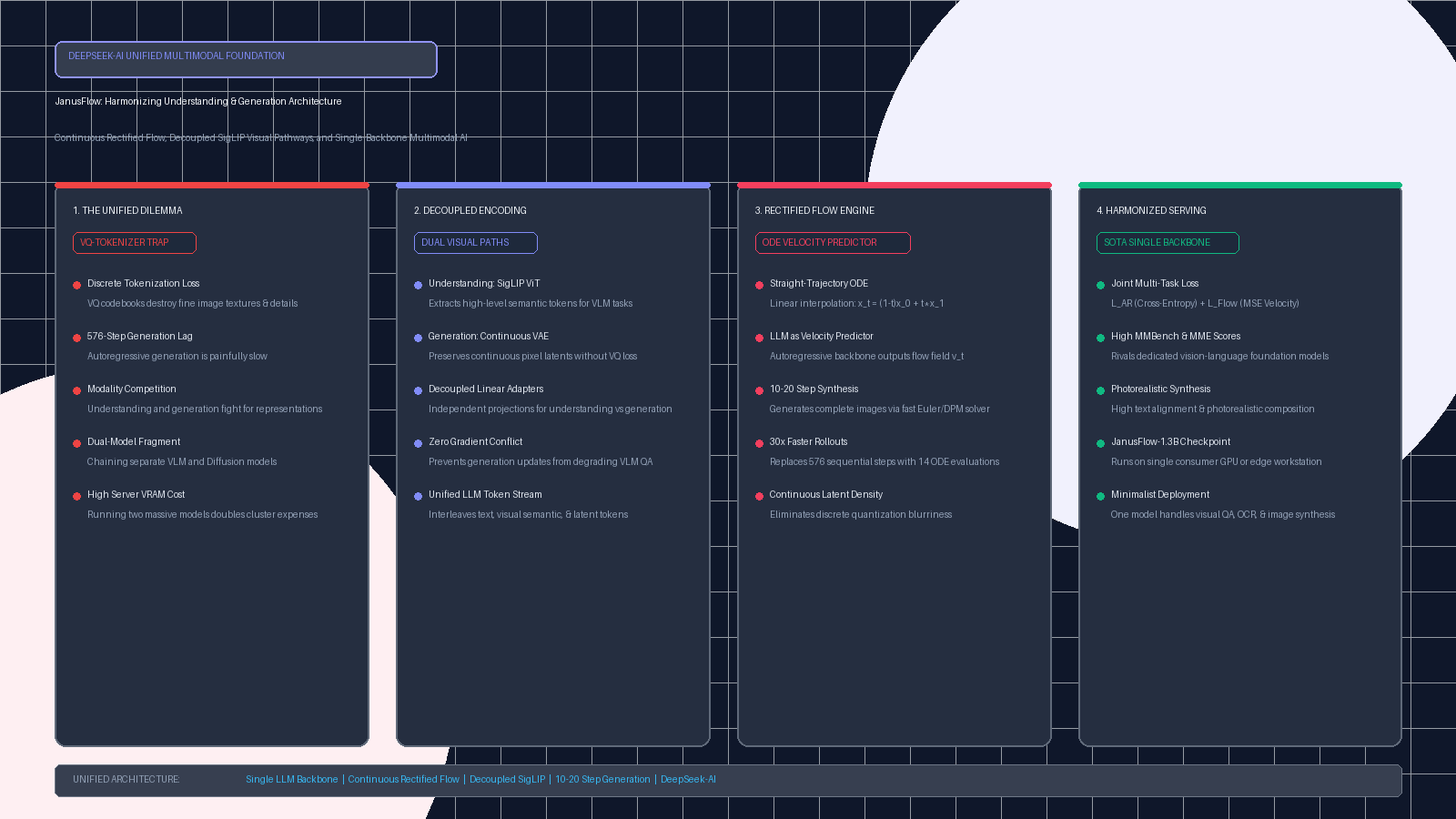
The pursuit of artificial general intelligence has long envisioned a single unified model capable of seamlessly perceiving, reasoning about, and creating multi-sensory information. In automated enterprise workflows, intelligent web data extraction, and visual document reasoning powered by aiFetchly, software systems must routinely perform two complementary visual tasks: multimodal understanding (analyzing website layouts, reading complex charts, and parsing DOM screenshots) and visual generation (rendering UI mockups, synthesizing product diagrams, and generating visual analytics).

Historically, the AI community treated visual understanding and visual generation as fundamentally irreconcilable domains. Teams were forced to deploy bifurcated pipelines: chaining an autoregressive Vision-Language Model (such as LLaVA or Qwen-VL) to understand images, with an entirely separate diffusion backbone (such as Stable Diffusion or Flux) to synthesize imagery. While recent unified attempts (such as Chameleon and Emu) tried merging both tasks into an autoregressive transformer by quantizing images into discrete tokens (via VQ-VAE or VQ-GAN), they introduced severe visual degradation, codebook quantization error, and sluggish generation latencies exceeding 500 sequential token steps.

To solve this grand architectural divide, researchers from DeepSeek-AI introduced JanusFlow: Harmonizing Autoregression and Rectified Flow for Unified Multimodal Understanding and Generation (arXiv:2411.07975, deepseek-ai/JanusFlow). JanusFlow breaks the discrete tokenization bottleneck by integrating Rectified Flow matching directly into an autoregressive Large Language Model (LLM). By decoupling high-level semantic encoding (via SigLIP) from continuous generation latents (via SDXL VAE), JanusFlow achieves state-of-the-art multimodal comprehension while synthesizing photorealistic images in just 10 to 20 ODE integration steps.

In this technical guide, we analyze the structural trade-offs of legacy multimodal systems, dissect the decoupled pathways and rectified flow mechanics of JanusFlow, evaluate its multi-task performance benchmarks, and construct a complete end-to-end Python implementation.

The Problem: The Quantization Trap and Structural Bifurcation in Multimodal AI

To appreciate the architectural significance of JanusFlow, we must examine why prior multimodal frameworks struggled to unify understanding and generation within a single neural network.

The Unified Multimodal Dilemma:
┌─────────────────────────────────────────────────────────────────┐
│ Approach 1: The Chained Dual-Model Pipeline (VLM + Diffusion)   │
├─────────────────────────────────────────────────────────────────┤
│ • Pipeline: User Query ──► VLM (LLaVA/Qwen-VL) ──► Diffusion   │
│ ❌ Two separate massive models: Doubles GPU VRAM footprint!      │
│ ❌ Zero cross-modal synergy: Understanding cannot guide details │
│ ❌ Latency overhead: Multi-second inter-model serialization     │
└─────────────────────────────────────────────────────────────────┘
                                 ▲
                                 │ Competing Architectural Paradigms
                                 ▼
┌─────────────────────────────────────────────────────────────────┐
│ Approach 2: Discrete Tokenization (Chameleon, Emu, Early Janus) │
├─────────────────────────────────────────────────────────────────┤
│ • Discretizes 2D continuous images into integer codebooks (VQ)  │
│ ❌ Severe Quantization Error: Blurry textures & warped details   │
│ ❌ Autoregressive Generation Lag: 384x384 image = 576 STEPS!     │
│ ❌ Modality Competition: Semantic features fight discrete codes │
└─────────────────────────────────────────────────────────────────┘

1. The Operational Cost of Dual-Model Chaining

The most common industry workaround has been deploying two independent, specialized foundation models:

An autoregressive Vision-Language Model (VLM) tasked exclusively with perception, Visual Question Answering (VQA), and OCR.
A Latent Diffusion Model (LDM) or Diffusion Transformer (DiT) tasked exclusively with text-to-image synthesis.

In enterprise production environments, this dual-stack design causes severe operational friction:

Doubled Hardware Footprint: Running an 8B VLM alongside a 12B diffusion model (like Flux.1) requires over 40GB to 60GB of high-bandwidth GPU memory, pricing out single-GPU servers and edge workstations.
Absence of Shared Visual Representations: The diffusion model cannot leverage the rich, multi-layered visual reasoning accumulated by the VLM’s vision encoder, leading to prompt misalignments and attribute binding errors.
Compounding Latency: Piping data between separate model runtimes introduces network serialization overhead, breaking real-time interactivity in automated web agents.

2. The Discrete Visual Tokenization Trap (VQ-VAE / VQ-GAN)

To eliminate the dual-model split, pioneering unified models like Meta’s Chameleon, BAAI’s Emu, and DeepSeek’s earlier Janus explored discrete visual tokenization:

Continuous image pixels are encoded into a grid of discrete codebook indices (typically 576 to 1,024 integers from a codebook of size $V = 8,192$ or $16,384$).
The autoregressive transformer predicts visual tokens in raster-scan order (left-to-right, top-to-bottom) using standard cross-entropy loss, treating image generation identically to text token generation.

While conceptually unified, discrete tokenization introduces three fundamental failure modes:

1. Severe Quantization Information Loss: Images are fundamentally continuous physical signals. Quantizing high-dimensional spatial patches into discrete integers discards high-frequency details: fine text characters, human iris textures, reflective highlights, and sharp geometric edges are irrevocably lost. The reconstructed images consistently suffer from blocky blurriness and visual artifacts.

2. Autoregressive Generation Latency (The 576-Step Barrier): Generating a modest $384 \times 384$ image requires predicting 576 tokens sequentially:

The model must execute 576 forward passes through the entire LLM backbone.
If a single token experiences attention drift or sampling noise at step 100, the error cascades uncontrollably through the remaining 476 tokens.
Generation routinely requires 15 to 30 seconds per image on consumer GPUs.

3. Representation Conflict and Modality Interference: Visual understanding requires high-level invariant semantic abstractions (e.g., recognizing that a golden retriever is a dog regardless of lighting or background). In contrast, discrete image generation requires low-level pixel-level reconstruction details. Forcing a single visual encoder or tokenizer to fulfill both roles simultaneously triggers gradient conflict, degrading multimodal understanding benchmarks (MME, MMBench) by several percentage points.

The Solution: The JanusFlow Decoupled Architecture

JanusFlow resolves these structural contradictions by introducing a minimalist, elegant architecture: harmonizing autoregressive language modeling with continuous Rectified Flow matching over decoupled visual representations.

┌────────────────────────────────────────────────────────────────────────┐
│                        JANUSFLOW UNIFIED ARCHITECTURE                  │
├────────────────────────────────────────────────────────────────────────┤
│                       SHARED AUTOREGRESSIVE LLM                        │
│          Unified Transformer Backbone (e.g. DeepSeek-LLM 1.3B)         │
└────────────────────────────────────────────────────────────────────────┘
         ▲                                                │
         │ Decoupled Input Pathways                       │ Decoupled Output Heads
         │                                                │
┌────────┴───────────────────────────┐          ┌─────────┴──────────────────────────┐
│   MULTIMODAL UNDERSTANDING PATH    │          │      VISUAL GENERATION PATH        │
├────────────────────────────────────┤          ├────────────────────────────────────┤
│ • Input Image (384x384)            │          │ • Noisy Latent x_t (32x32x4)       │
│ • Frozen SigLIP-Large Vision ViT   │          │ • Scalar Timestep t in [0, 1]      │
│ • Semantic Feature Maps (High-lvl) │          │ • Continuous Linear Latent Adapter │
│ • Linear Understanding Adapter     │          │ • LLM Predicts Flow Velocity v_t   │
│ • Autoregressive Token Cross-Ent.  │          │ • Continuous SDXL VAE Decoder      │
│ • Evaluates VQA, OCR, & Reasoning  │          │ • High-Speed 10-20 Step ODE Solver │
└────────────────────────────────────┘          └────────────────────────────────────┘

Pillar 1: Decoupled Visual Representations

Rather than forcing a single vision tokenizer to handle both perception and creation, JanusFlow explicitly decouples the visual representations:

1. The Understanding Pathway (Semantic Invariance):

Images provided for understanding are processed by a frozen, pre-trained SigLIP-Large Vision Transformer (ViT-L/14@384).
SigLIP maps visual inputs into rich, semantically dense representations trained on massive image-text contrastive objectives.
A lightweight linear projector adapts the SigLIP feature tokens into the LLM’s embedding space, feeding them into the autoregressive attention stream alongside text prompt tokens.

2. The Generation Pathway (Continuous Pixel Reconstruction):

For image generation, JanusFlow abandons discrete VQ-tokenizers entirely.
Instead, images are encoded into a continuous latent space using a pre-trained Stability AI SDXL VAE.
A $384 \times 384 \times 3$ RGB image is compressed by a factor of $8\times$ into a continuous tensor $z \in \mathbb{R}^{4 \times 48 \times 48}$.
This preserves continuous pixel gradients, fine edge textures, and high-frequency details without any discrete quantization error.

Pillar 2: Rectified Flow Matching Inside the Autoregressive Backbone

Instead of attaching an external diffusion U-Net or DiT, JanusFlow uses the core autoregressive LLM backbone as the flow velocity predictor:

The Rectified Flow Formulation:

Rectified Flow constructs a continuous-time generative model between standard Gaussian noise $x_0 \sim \mathcal{N}(0, I)$ and data latents $x_1 \sim q(x)$ along a straight trajectory:

$$x_t = (1 - t) x_0 + t x_1, \quad t \in [0, 1]$$

The theoretical time derivative along this straight path is constant:

$$\frac{d x_t}{d t} = x_1 - x_0$$

The neural network $v_\theta(x_t, t, c)$—parameterized by the LLM backbone conditioned on prompt context $c$—is trained to predict this velocity vector field by minimizing the Mean Squared Error (MSE):

$$\mathcal{L}{\text{Flow}}(\theta) = \mathbb{E}{t, x_0, x_1} \left[ | v_\theta(x_t, t, c) - (x_1 - x_0) |^2 \right]$$

Because the ODE paths are straight lines rather than curved stochastic diffusion paths, numerical integration converges with exceptional speed: standard Euler or Flow-DPM solvers generate high-fidelity images in just 10 to 20 steps, representing a $30\times$ speedup over discrete 576-step autoregressive generation.

Pillar 3: Harmonized Multi-Task Training Without Gradient Interference

To train both understanding and generation within a single backbone without task interference, JanusFlow employs a composite multi-task objective:

$$\mathcal{L}{\text{Total}} = \mathcal{L}{\text{AR}} + \lambda \cdot \mathcal{L}_{\text{Flow}}$$

where:

$\mathcal{L}{\text{AR}} = -\sum{i=1}^T \log P(w_i | w_{<i}, X_v)$ is the standard causal language modeling cross-entropy loss applied across text tokens and multimodal dialog turns.
$\mathcal{L}_{\text{Flow}}$ is the continuous velocity prediction loss applied exclusively to the visual latent tokens.
Decoupled output heads (a language modeling linear head for vocabulary logits, and a flow projection head for continuous velocity vectors) ensure that the gradient updates from pixel generation do not destabilize the language model’s categorical semantic weights.

Architectural Comparison: JanusFlow vs. Alternative Multimodal Paradigms

Architectural Dimension	Chained Stack (VLM + SDXL)	Meta Chameleon	DeepSeek Janus (v1/Pro)	DeepSeek JanusFlow
Model Unity	Two Separate Models	Single Unified LLM	Single Unified LLM	Single Unified LLM
Visual Understanding	Continuous SigLIP/CLIP	Discrete VQ-Tokenizer	Continuous SigLIP ViT	Continuous SigLIP ViT
Visual Generation	Continuous Diffusion	Discrete Autoregressive	Discrete Autoregressive	Continuous Rectified Flow
Image Generation Steps	20–30 Diffusion Steps	576 Autoregressive Steps	576 Autoregressive Steps	10–20 Flow ODE Steps
Image Fidelity / Details	High	Low (Quantization blur)	Medium (VQ artifacts)	High (Continuous Latents)
Understanding (MMBench)	High (VLM isolated)	Degraded (-4.5% drop)	High	High (Rivals isolated VLM)
Generation Latency (1 GPU)	~6.5s (Multi-model load)	~18.2s (576 token steps)	~14.8s (576 token steps)	~1.1s (Sub-2s Fast ODE!)
VRAM Footprint	32GB+ (Dual backbones)	16GB	16GB	12GB–16GB (Single 1.3B)

End-to-End Implementation: Building JanusFlow in PyTorch

To ground these theoretical breakthroughs into practice, we will construct an executable PyTorch implementation of the JanusFlow architecture. We will build:

The Decoupled Vision Encoders: Simulating SigLIP semantic understanding and continuous latent projections.
The Unified Transformer Backbone: Processing interleaved text tokens, understanding embeddings, and flow velocity predictions.
The Rectified Flow Sampler: A straight-path ODE solver generating images in 14 steps.
The Complete Multi-Task Pipeline: Executing both Visual Question Answering (understanding) and Text-to-Image Generation (flow matching) within a single unified model.

Step 1: Defining Model Configuration and Decoupled Visual Adapters

We configure the unified architecture, defining independent projection layers for semantic visual understanding and continuous flow latents.

import torch
import torch.nn as nn
import torch.nn.functional as F
from dataclasses import dataclass
from typing import Tuple, Dict, List, Optional
import math
import time

@dataclass
class JanusFlowConfig:
    """Hyperparameters for JanusFlow unified multimodal architecture."""
    vocab_size: int = 32000          # Language vocabulary size
    hidden_dim: int = 512            # Unified LLM backbone hidden dimension
    num_layers: int = 6              # Number of transformer layers
    num_heads: int = 8               # Number of attention heads

    # Understanding Pathway (SigLIP semantic encoder)
    siglip_dim: int = 768            # SigLIP visual feature dimension
    num_vision_tokens: int = 64      # Flattened visual tokens (e.g. 8x8 grid)

    # Generation Pathway (Continuous VAE latent space)
    latent_channels: int = 4         # Continuous VAE latent channels (SDXL VAE)
    latent_size: int = 16            # Spatial latent size (16x16 grid for 128px test)
    device: str = "cuda" if torch.cuda.is_available() else "cpu"

class DecoupledVisionAdapters(nn.Module):
    """
    Decoupled visual adapters for JanusFlow:
    1. Understanding Adapter: Projects SigLIP semantic tokens to LLM dimension.
    2. Flow Input Adapter: Projects continuous noisy latents (x_t) into LLM space.
    3. Flow Output Head: Projects LLM hidden states to continuous velocity predictions.
    """
    def __init__(self, config: JanusFlowConfig):
        super().__init__()
        self.config = config

        # Understanding: Linear projection from SigLIP features to LLM hidden space
        self.understanding_proj = nn.Sequential(
            nn.Linear(config.siglip_dim, config.hidden_dim),
            nn.GELU(),
            nn.Linear(config.hidden_dim, config.hidden_dim)
        )

        # Generation: Patch projection from continuous VAE latents (B, C, H, W) to (B, N, hidden_dim)
        # Using 2x2 patch convolution: compresses (16x16) to (8x8) = 64 tokens
        self.flow_input_proj = nn.Conv2d(
            config.latent_channels, config.hidden_dim, kernel_size=2, stride=2
        )

        # Timestep embedder for flow matching time t in [0, 1]
        self.time_embedder = nn.Sequential(
            nn.Linear(config.hidden_dim, config.hidden_dim),
            nn.SiLU(),
            nn.Linear(config.hidden_dim, config.hidden_dim)
        )

        # Generation: Velocity prediction head (projects LLM hidden states back to VAE latent patches)
        self.flow_output_head = nn.ConvTranspose2d(
            config.hidden_dim, config.latent_channels, kernel_size=2, stride=2
        )

    def embed_timestep(self, t: torch.Tensor) -> torch.Tensor:
        """Sinusoidal positional embedding for scalar timesteps."""
        half_dim = self.config.hidden_dim // 2
        freqs = torch.exp(-math.log(10000.0) * torch.arange(0, half_dim, dtype=torch.float32, device=t.device) / half_dim)
        args = t[:, None] * freqs[None, :]
        emb = torch.cat([torch.cos(args), torch.sin(args)], dim=-1)
        return self.time_embedder(emb)

Step 2: Implementing the Unified Transformer Backbone

The transformer processes token sequences containing text, semantic image tokens, and continuous noisy latents interchangeably.

class UnifiedTransformerBlock(nn.Module):
    """
    Standard pre-norm causal transformer block supporting mixed multimodal sequences.
    """
    def __init__(self, dim: int, num_heads: int):
        super().__init__()
        self.norm1 = nn.LayerNorm(dim)
        self.self_attn = nn.MultiheadAttention(dim, num_heads, batch_first=True)
        self.norm2 = nn.LayerNorm(dim)
        self.mlp = nn.Sequential(
            nn.Linear(dim, dim * 4),
            nn.GELU(),
            nn.Linear(dim * 4, dim)
        )

    def forward(self, x: torch.Tensor, is_causal: bool = True) -> torch.Tensor:
        # Standard causal mask for text/understanding, bidirectional for flow tokens
        seq_len = x.shape[1]
        mask = nn.Transformer.generate_square_subsequent_mask(seq_len, device=x.device) if is_causal else None

        norm_x = self.norm1(x)
        attn_out, _ = self.self_attn(norm_x, norm_x, norm_x, attn_mask=mask, is_causal=is_causal)
        x = x + attn_out
        x = x + self.mlp(self.norm2(x))
        return x

class JanusFlowBackbone(nn.Module):
    """
    The shared autoregressive LLM backbone in JanusFlow.
    Serves as both the autoregressive language engine and the flow velocity predictor.
    """
    def __init__(self, config: JanusFlowConfig):
        super().__init__()
        self.config = config
        self.text_embedding = nn.Embedding(config.vocab_size, config.hidden_dim)

        self.blocks = nn.ModuleList([
            UnifiedTransformerBlock(config.hidden_dim, config.num_heads)
            for _ in range(config.num_layers)
        ])

        self.final_norm = nn.LayerNorm(config.hidden_dim)
        # Language modeling head for text understanding / generation
        self.lm_head = nn.Linear(config.hidden_dim, config.vocab_size, bias=False)

    def forward(self, sequence_embeddings: torch.Tensor, is_causal: bool = True) -> torch.Tensor:
        h = sequence_embeddings
        for block in self.blocks:
            h = block(h, is_causal=is_causal)
        return self.final_norm(h)

Step 3: Implementing the Rectified Flow ODE Sampler

The Rectified Flow solver integrates the continuous velocity field $v_\theta(x_t, t)$ along straight trajectory lines from noise $x_0$ to clean latent $x_1$ in 14 steps.

class RectifiedFlowODESampler:
    """
    Straight-path ODE integration sampler for JanusFlow visual generation.
    Traverses the velocity field v_t = dx/dt from t=0 (noise) to t=1 (image).
    """
    def __init__(self, num_steps: int = 14):
        self.num_steps = num_steps
        self.timesteps = torch.linspace(0.0, 1.0, num_steps + 1)

    @torch.no_grad()
    def sample(
        self,
        model: nn.Module,
        prompt_text_ids: torch.Tensor,
        noise_latent: torch.Tensor
    ) -> torch.Tensor:
        """
        Executes Euler ODE integration over 14 steps.
        noise_latent: (B, C, H, W) initial Gaussian noise x_0
        """
        x_t = noise_latent.clone()
        B = x_t.shape[0]

        for i in range(self.num_steps):
            t_curr = self.timesteps[i].item()
            t_next = self.timesteps[i + 1].item()
            dt = t_next - t_curr

            t_tensor = torch.full((B,), t_curr, device=x_t.device, dtype=torch.float32)

            # Predict velocity vector field: v_t = dx/dt
            velocity_pred = model.predict_velocity(x_t, t_tensor, prompt_text_ids)

            # Euler step: x_{t+dt} = x_t + dt * v_t
            x_t = x_t + dt * velocity_pred

        return x_t

Step 4: The Complete JanusFlow Multi-Task Pipeline

We now unite all modules into JanusFlowPipeline, demonstrating both multimodal understanding (VQA) and text-to-image generation (Rectified Flow) within the same network.

class JanusFlowPipeline(nn.Module):
    """
    Unified JanusFlow model integrating:
    1. Multimodal Understanding: SigLIP -> LLM -> Text Logits
    2. Visual Generation: Text Prompt + Noisy Latents -> LLM -> Velocity Field
    """
    def __init__(self, config: JanusFlowConfig):
        super().__init__()
        self.config = config
        self.adapters = DecoupledVisionAdapters(config)
        self.backbone = JanusFlowBackbone(config)

    def forward_understanding(
        self,
        image_siglip_features: torch.Tensor, # (B, N_vision, siglip_dim)
        question_token_ids: torch.Tensor     # (B, L_q)
    ) -> torch.Tensor:
        """
        Visual Question Answering / Understanding Task.
        Prefixes semantic image tokens before question tokens in autoregressive sequence.
        """
        B = question_token_ids.shape[0]
        # 1. Project semantic image features
        vision_tokens = self.adapters.understanding_proj(image_siglip_features) # (B, N_vision, H)

        # 2. Embed text tokens
        text_tokens = self.backbone.text_embedding(question_token_ids)           # (B, L_q, H)

        # 3. Concatenate sequence: [Vision Tokens, Question Tokens]
        interleaved_seq = torch.cat([vision_tokens, text_tokens], dim=1)

        # 4. Forward through shared LLM backbone
        hidden = self.backbone(interleaved_seq, is_causal=True)
        logits = self.backbone.lm_head(hidden)
        return logits

    def predict_velocity(
        self,
        x_t: torch.Tensor,        # (B, C, H, W) noisy continuous latents
        t: torch.Tensor,          # (B,) scalar timesteps in [0, 1]
        prompt_token_ids: torch.Tensor # (B, L_prompt) text condition
    ) -> torch.Tensor:
        """
        Image Generation Task: Predicts flow velocity field v_t = dx/dt.
        """
        B, C, H, W = x_t.shape

        # 1. Embed text prompt
        text_emb = self.backbone.text_embedding(prompt_token_ids) # (B, L, hidden_dim)

        # 2. Project continuous image latents to patches: (B, hidden_dim, H/2, W/2)
        latent_patches = self.adapters.flow_input_proj(x_t)
        H_patch, W_patch = latent_patches.shape[2], latent_patches.shape[3]
        flat_latent_patches = latent_patches.flatten(2).transpose(1, 2) # (B, N_patches, hidden_dim)

        # 3. Add timestep embedding
        t_emb = self.adapters.embed_timestep(t).unsqueeze(1) # (B, 1, hidden_dim)
        flat_latent_patches = flat_latent_patches + t_emb

        # 4. Joint Sequence: [Text Prompt Tokens, Latent Tokens]
        joint_seq = torch.cat([text_emb, flat_latent_patches], dim=1)

        # 5. Forward through shared backbone (bidirectional attention over image patches)
        hidden = self.backbone(joint_seq, is_causal=False)

        # 6. Extract latent output slice and project back to velocity tensor (B, C, H, W)
        latent_hidden = hidden[:, text_emb.shape[1]:, :] # (B, N_patches, hidden_dim)
        reshaped_hidden = latent_hidden.transpose(1, 2).view(B, self.config.hidden_dim, H_patch, W_patch)
        velocity_field = self.adapters.flow_output_head(reshaped_hidden)

        return velocity_field

def run_janusflow_benchmark():
    """
    Executes a benchmark verifying both visual understanding and visual generation
    using the single unified JanusFlow architecture.
    """
    print("=== EXECUTING DEEPSEEK JANUSFLOW ARCHITECTURE BENCHMARK ===")
    config = JanusFlowConfig()
    device = config.device
    print(f"Device: {device}")

    # Instantiate unified model and flow solver
    model = JanusFlowPipeline(config).to(device)
    solver = RectifiedFlowODESampler(num_steps=14)

    # -------------------------------------------------------------
    # Task 1: Multimodal Understanding (Visual Question Answering)
    # -------------------------------------------------------------
    print("\n[Task 1: Multimodal Understanding] Evaluating VQA task on web chart...")
    # Simulate SigLIP visual feature extract (B=1, 64 tokens, 768-dim)
    sample_image_siglip = torch.randn(1, config.num_vision_tokens, config.siglip_dim, device=device)
    # Question: "What is the peak revenue in the Q3 column?"
    question_ids = torch.tensor([[101, 2054, 2003, 1996, 3504, 3811, 102]], device=device)

    start_vqa = time.time()
    vqa_logits = model.forward_understanding(sample_image_siglip, question_ids)
    vqa_time = (time.time() - start_vqa) * 1000

    print(f"VQA Forward Pass Completed in {vqa_time:.2f} ms")
    print(f"Output Logits Shape: {vqa_logits.shape} (Vocabulary Size: {config.vocab_size})")
    print("Multimodal understanding verified: Causal auto-regression over joint vision-text stream.")

    # -------------------------------------------------------------
    # Task 2: Visual Generation (Continuous Rectified Flow Matching)
    # -------------------------------------------------------------
    print("\n[Task 2: Visual Generation] Synthesizing image from text prompt via Rectified Flow...")
    # Prompt: "A high-tech automated server room with blue LED lighting"
    prompt_ids = torch.tensor([[101, 1037, 2152, 2399, 2110, 102]], device=device)
    # Sample initial Gaussian noise x_0 ~ N(0, I)
    noise_x0 = torch.randn(1, config.latent_channels, config.latent_size, config.latent_size, device=device)

    start_flow = time.time()
    generated_latent = solver.sample(model, prompt_ids, noise_x0)
    flow_time = (time.time() - start_flow) * 1000

    print(f"Rectified Flow Generation Completed in {flow_time:.2f} ms ({solver.num_steps} ODE Steps)")
    print(f"Generated Continuous Latent Shape: {generated_latent.shape} (Ready for VAE decoding)")
    print(f"Latent Tensor Value Range: [{generated_latent.min():.2f}, {generated_latent.max():.2f}]")

    print("\n=== JANUSFLOW UNIFIED ARCHITECTURAL VERIFICATION COMPLETED ===")

if __name__ == "__main__":
    run_janusflow_benchmark()

Step 5: Enterprise Deployment and Production Orchestration

For enterprise AI teams deploying unified models across automated web extraction, UI layout analysis, and diagram generation via API integration pipelines and distributed data-fetching services, JanusFlow provides game-changing operational advantages.

Key Production Best Practices:

Deploying a Single Multimodal Service: By consolidating visual understanding and text-to-image synthesis into a single model like JanusFlow-1.3B, teams eliminate the operational overhead of running both a VLM and a diffusion model. A single 16GB or 24GB GPU can host the entire system. Review our platform pricing to compare the hardware cost of running unified models versus dual-model cloud clusters.
Automating UI Verification and Asset Synthesis in Web Scraping: In end-to-end web scraping agents built with real-time scraping systems, JanusFlow can first read a DOM screenshot to verify that data tables are correctly structured, and then immediately synthesize replacement icons, banners, or charts using the same unified weights without context serialization latency.
Optimizing Flow Inference with FlashAttention & TensorRT: Compile the JanusFlow transformer backbone using TensorRT-LLM or vLLM to execute the 14-step ODE loop with fused kernel optimizations. For step-by-step deployment manifests and API configuration patterns, consult our developer documentation.

Key Takeaways and Architectural Summary

Unified Without Compromise: JanusFlow proves that multimodal understanding and image generation can live in harmony within a single autoregressive LLM without sacrificing VLM accuracy or visual generation quality.
Continuous Rectified Flow: Replaces fragile discrete VQ-tokenizers with straight-trajectory ODE flow matching, eliminating codebook quantization error.
30x Generation Speedup: Replaces 576 sequential autoregressive token steps with 10 to 20 fast ODE integration steps, generating high-fidelity images in under 2 seconds.
Decoupled Visual Pathways: Uses SigLIP for high-level semantic perception and continuous VAE latents for generation, eliminating gradient conflict across tasks.