Inference-Optimal Scaling: Why Over-Training LLMs Wins
The Problem: The Chinchilla Fallacy in Production AI
In modern enterprise generative AI, high-concurrency browser automation agents, and automated web extraction platforms like AiFetchly, foundation model economics are governed by two distinct cost centers: pre-training compute and recurring inference serving.
Historically, the machine learning industry treated compute allocation through the lens of static pre-training scaling laws.
The Evolution of Scaling Laws
- Kaplan et al. (OpenAI, 2020): Proposed that when expanding a compute budget $C$, model parameters $N$ should scale much faster than training data tokens $D$: $$N \propto C^{0.73}, \quad D \propto C^{0.27}$$ This led the industry to build massive, severely under-trained architectures—most notably GPT-3 (175 billion parameters trained on only 300 billion tokens, or a ratio $D/N \approx 1.7$).
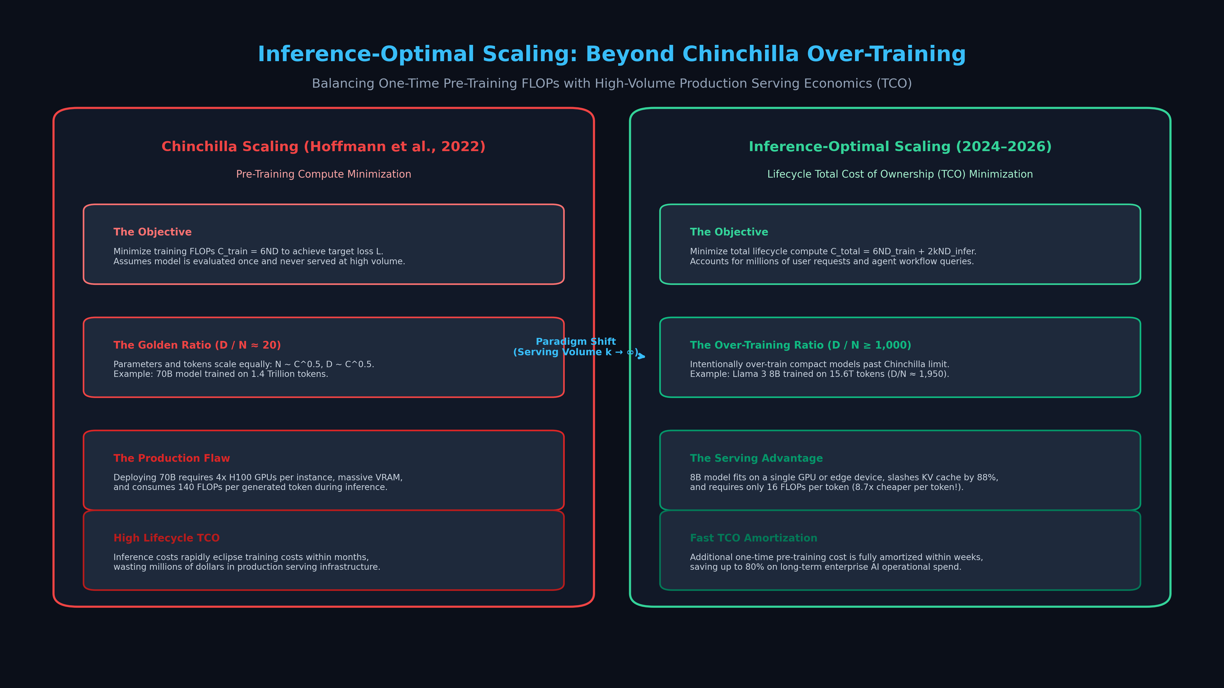
- Hoffmann et al. (DeepMind Chinchilla, 2022): Corrected Kaplan’s formulation, establishing that for compute-optimal pre-training, parameters and tokens must scale in equal proportion: $$N \propto C^{0.5}, \quad D \propto C^{0.5}$$ Under Chinchilla’s golden ratio, a model should consume approximately 20 tokens per parameter ($D/N \approx 20$). For example, a 70B parameter model is compute-optimal when trained on 1.4 trillion tokens.
The Fatal Flaw of Chinchilla in Production
While Chinchilla scaling is mathematically rigorous, it solves a very narrow optimization problem: minimizing pre-training FLOPs to achieve a target loss.
Crucially, Chinchilla assumes the trained model will be evaluated once and never served at scale.
In real-world enterprise software, this assumption completely breaks down:
- The Serving FLOP Penalty: The computational cost of generating a single output token scales linearly with parameter count: $$\text{FLOPs per token} \approx 2N$$ Generating one token with a 70B model requires 140 billion FLOPs, whereas generating that same token with an 8B model requires only 16 billion FLOPs—an 8.75x computational difference on every single output token.
- Hardware Footprint and High-Bandwidth Memory (HBM): Serving a 70B model requires at least 4x NVIDIA H100 (80GB) GPUs or expensive 8-GPU tensor-parallel nodes. An 8B model fits comfortably on a single GPU or local workstation, consuming an order of magnitude less power and DRAM.
- The Lifecycle Cost Reversal: In applications where an AI model generates hundreds of billions or trillions of tokens over its operational lifetime, inference costs dwarf pre-training costs by $10\times$ to $100\times$ within months.
Optimizing solely for pre-training efficiency results in catastrophic operational waste in production.
The Architecture: Total Cost of Ownership (TCO) Scaling Formulation
To resolve the pre-training versus serving imbalance, frontier labs transitioned to Inference-Optimal Scaling Laws (Sardana & Frankle, 2023; Meta Llama 3 Team, 2024).
The fundamental thesis is straightforward: It is economically optimal to spend significantly more compute during pre-training to make the resulting model smaller, faster, and cheaper during downstream inference.
The Paradigm Shift in AI Compute Allocation:
┌─────────────────────────┬─────────────────────────┬─────────────────────────┐
│ Metric / Property       │ Chinchilla-Optimal      │ Inference-Optimal       │
├─────────────────────────┼─────────────────────────┼─────────────────────────┤
│ Optimization Target     │ Min Pre-Training FLOPs  │ Min Total Lifecycle TCO │
│ Typical D / N Ratio     │ ~20 Tokens / Parameter  │ 1,000–2,000+ Tokens / P │
│ Example Configuration   │ 70B Params on 1.4T Toks │ 8B Params on 15.6T Toks │
│ Production Footprint    │ 4–8 GPUs (160–320 GB)   │ 1 GPU (16–24 GB)        │
│ Serving Cost per Token  │ 100% Baseline           │ 11.4% (8.75x Cheaper)   │
│ Target Use Case         │ Academic / Low-Volume   │ High-Volume SaaS & Edge │
└─────────────────────────┴─────────────────────────┴─────────────────────────┘ The Total Lifecycle Compute Formulation
Let $N$ be model parameter count, $D_{\text{train}}$ be training tokens, and $D_{\text{infer}}$ be the total cumulative volume of inference tokens the model is expected to serve over its production lifespan.
The total lifecycle compute $\mathcal{C}_{\text{total}}$ is:
$$\mathcal{C}{\text{total}}(N, D{\text{train}}, D_{\text{infer}}) = \underbrace{6 N D_{\text{train}}}{\text{Pre-Training FLOPs}} + \underbrace{2 N D{\text{infer}}}_{\text{Inference FLOPs}}$$
When inference demand $D_{\text{infer}}$ is projected to be large:
- The marginal cost of increasing $D_{\text{train}}$ is paid once by the foundation model builder.
- The cost savings from shrinking $N$ are harvested on every single downstream user query.
The Over-Training Power Law
Does a language model continue to learn when trained far past the Chinchilla boundary ($D/N \gg 20$)?
Empirical loss curves follow a modified power law:
$$L(N, D) = E + \frac{A}{N^\alpha} + \frac{B}{D^\beta}$$
While returns on training tokens diminish logarithmically, loss continues to decline monotonically even at $D/N > 2,000$. More importantly, an over-trained small model matches or exceeds the downstream capabilities of a larger under-trained model across reasoning, coding, and factual retrieval benchmarks.
Mathematical Mechanics: The Break-Even Crossover and Amortization Dynamics
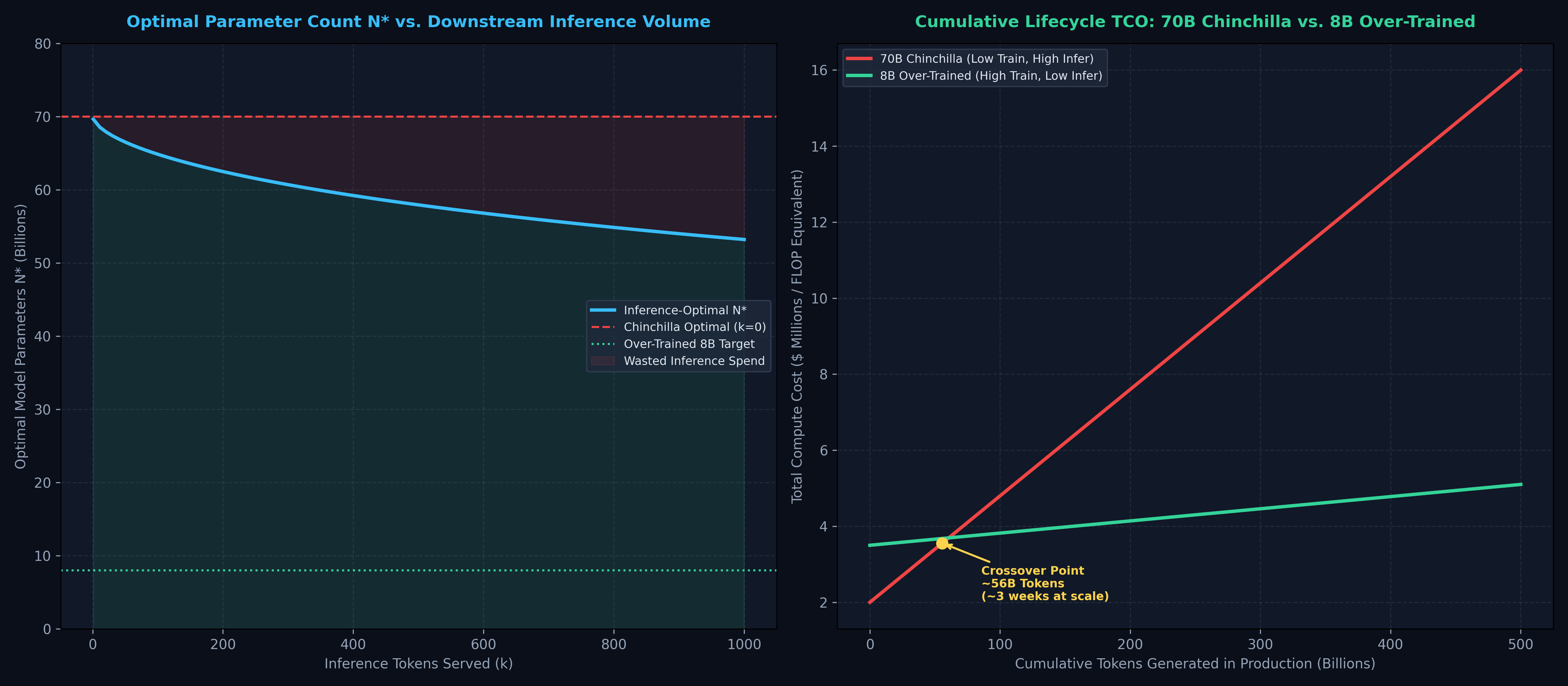
To determine whether an engineering team should deploy a larger Chinchilla-optimal model or train an over-trained compact model, we calculate the Break-Even Crossover Volume.
1. Mathematical Derivation of Crossover Volume
Consider two candidate models that achieve identical task loss:
- Model 1 (Large Chinchilla Model): $N_1 = 70\text{B}$ parameters, $D_1 = 1.4\text{T}$ training tokens.
- Model 2 (Over-Trained Small Model): $N_2 = 8\text{B}$ parameters, $D_2 = 15.6\text{T}$ training tokens.
The difference in upfront pre-training compute is:
$$\Delta \mathcal{C}_{\text{train}} = 6 \left( N_2 D_2 - N_1 D_1 \right)$$
Plugging in parameter numbers:
- $\mathcal{C}_{\text{train}}(M_1) = 6 \times (70 \times 10^9) \times (1.4 \times 10^{12}) \approx 5.88 \times 10^{23} \text{ FLOPs}$
- $\mathcal{C}_{\text{train}}(M_2) = 6 \times (8 \times 10^9) \times (15.6 \times 10^{12}) \approx 7.49 \times 10^{23} \text{ FLOPs}$
- $\Delta \mathcal{C}_{\text{train}} \approx 1.61 \times 10^{23} \text{ FLOPs}$ (Over-training $M_2$ requires ~27% more pre-training compute).
The inference compute savings per generated token is:
$$\Delta \mathcal{C}_{\text{infer/token}} = 2 (N_1 - N_2) = 2 \times (70 - 8) \times 10^9 = 1.24 \times 10^{11} \text{ FLOPs/token}$$
The break-even crossover token threshold $D^*$ where Model 2 becomes strictly cheaper than Model 1 is:
$$D^* = \frac{\Delta \mathcal{C}{\text{train}}}{\Delta \mathcal{C}{\text{infer/token}}} = \frac{1.61 \times 10^{23}}{1.24 \times 10^{11}} \approx 1.30 \times 10^{12} \text{ tokens}$$
1.3 Trillion inference tokens is the pure theoretical compute crossover. In practice, because hardware serving efficiency favors smaller models, the real financial dollar crossover occurs far earlier.
2. The Memory Bandwidth Multiplier
In autoregressive inference, generating tokens is strictly memory-bandwidth bound rather than compute bound. The GPU must transport every parameter weight from High-Bandwidth Memory (HBM) to on-chip registers for each token generated:
$$\text{Memory Bandwidth Demand} = 2N \text{ Bytes per token (in 16-bit)}$$
- For a 70B model, the memory bus must stream 140 GB of weights per token.
- For an 8B model, the bus streams only 16 GB of weights per token.
Because smaller models fit comfortably in on-chip caches and single-GPU SRAM, an over-trained 8B model delivers 4x to 6x higher throughput per GPU dollar than a 70B model. Factoring in cloud hosting, energy, and networking expenses, the true financial crossover point drops to under 50 billion tokens—a milestone high-traffic enterprise applications cross in just weeks.
Practical Implementation: The Enterprise TCO & Crossover Calculator
The following Python tool enables machine learning infrastructure leaders to calculate the exact financial crossover point between Chinchilla-optimal and over-trained model configurations:
def calculate_scaling_tco(
    n_large_b: float,          # Size of large model in billions (e.g., 70.0)
    d_large_t: float,          # Training tokens for large model in trillions (e.g., 1.4)
    n_small_b: float,          # Size of small model in billions (e.g., 8.0)
    d_small_t: float,          # Training tokens for small model in trillions (e.g., 15.6)
    gpu_cost_per_hour: float,  # Cost per H100 GPU hour ($)
    h100_tflops: float = 989.0 # Peak FP16 Tensor Core TFLOPS
):
    """
    Computes upfront training costs, per-million inference costs,
    and the break-even token crossover point.
    """
    # 1. Calculate Pre-training FLOPs
    flops_train_large = 6.0 * (n_large_b * 1e9) * (d_large_t * 1e12)
    flops_train_small = 6.0 * (n_small_b * 1e9) * (d_small_t * 1e12)

    # Effective training MFU assumed at 40%
    eff_flops_per_sec = h100_tflops * 1e12 * 0.40
    gpu_hours_large = flops_train_large / (eff_flops_per_sec * 3600.0)
    gpu_hours_small = flops_train_small / (eff_flops_per_sec * 3600.0)

    train_cost_large = gpu_hours_large * gpu_cost_per_hour
    train_cost_small = gpu_hours_small * gpu_cost_per_hour

    # 2. Calculate Serving FLOPs per Million Tokens
    # 2 * N FLOPs per token * 1,000,000 tokens
    flops_per_m_large = 2.0 * (n_large_b * 1e9) * 1e6
    flops_per_m_small = 2.0 * (n_small_b * 1e9) * 1e6

    # Serving MFU assumed at 25% (memory bandwidth bound)
    serving_flops_per_sec = h100_tflops * 1e12 * 0.25
    infer_cost_per_m_large = (flops_per_m_large / (serving_flops_per_sec * 3600.0)) * gpu_cost_per_hour
    infer_cost_per_m_small = (flops_per_m_small / (serving_flops_per_sec * 3600.0)) * gpu_cost_per_hour

    # 3. Calculate Crossover Token Volume
    delta_train_cost = train_cost_small - train_cost_large
    delta_infer_per_m = infer_cost_per_m_large - infer_cost_per_m_small

    crossover_m_tokens = delta_train_cost / delta_infer_per_m if delta_infer_per_m > 0 else float('inf')
    crossover_b_tokens = crossover_m_tokens / 1e3

    return {
        "large_model_train_cost": round(train_cost_large, 2),
        "small_model_train_cost": round(train_cost_small, 2),
        "delta_training_investment": round(delta_train_cost, 2),
        "large_infer_cost_per_1m": round(infer_cost_per_m_large, 5),
        "small_infer_cost_per_1m": round(infer_cost_per_m_small, 5),
        "crossover_billion_tokens": round(crossover_b_tokens, 2)
    }

# Example run: Comparing 70B Chinchilla vs 8B Over-Trained on H100 GPUs ($3.00/hr)
analysis = calculate_scaling_tco(
    n_large_b=70.0, d_large_t=1.4,
    n_small_b=8.0, d_small_t=15.6,
    gpu_cost_per_hour=3.00
)

print("TCO Analysis Summary:")
for k, v in analysis.items():
print(f" {k}: {v}") Empirical Case Studies: Llama 3, Gemma 2, and DeepSeek
The transition to inference-optimal scaling is evident across the frontier open-weights ecosystem:
Industry Over-Training Empirical Comparison:
┌─────────────────────┬──────────────┬──────────────┬──────────┬────────────────┬──────────────────┐
│ Model               │ Parameters   │ Training     │ D / N    │ MMLU           │ Hardware         │
│                     │ (N)          │ Tokens (D)   │ Ratio    │ Score          │ Footprint        │
├─────────────────────┼──────────────┼──────────────┼──────────┼────────────────┼──────────────────┤
│ Chinchilla Baseline │ 70.0 Billion │ 1.4 Trillion │ 20.0     │ 67.5%          │ 4x 80GB GPUs     │
│ Llama 2 70B         │ 68.9 Billion │ 2.0 Trillion │ 29.0     │ 68.9%          │ 4x 80GB GPUs     │
│ Llama 3 8B          │ 8.0 Billion  │ 15.6 Trill.  │ 1,950.0  │ 68.4%          │ 1x 24GB GPU      │
│ Gemma 2 9B          │ 9.2 Billion  │ 8.0 Trillion │ 869.5    │ 71.3%          │ 1x 24GB GPU      │
│ DeepSeek-Coder-V2   │ 16.0 Billion │ 10.2 Trill.  │ 637.5    │ 79.2% (Coding) │ 1x 48GB GPU      │
└─────────────────────┴──────────────┴──────────────┴──────────┴────────────────┴──────────────────┘ The empirical results reveal a historic milestone: Llama 3 8B ($D/N = 1,950$) matches the performance of Llama 2 70B while requiring an 8.75x lower computational budget on every single inference pass.
Strategic Recommendations for Production Deployments
When deciding how to allocate compute across pre-training and inference in your organization:
1. Apply the Rule of Projected Lifetime Volume
- The Chinchilla Zone ($D_{\text{infer}} < 10\text{B}$ tokens): If your model is an experimental research prototype, an internal proof-of-concept, or a low-volume niche batch-job, adhere to Chinchilla scaling. Minimizing training compute saves capital.
- The Over-Training Zone ($D_{\text{infer}} \ge 50\text{B}$ tokens): If the model will power customer-facing SaaS, live search agents, or public APIs, over-train an 8B or 14B model by $50\times$ to $100\times$ beyond the Chinchilla ratio. The initial training premium will amortize within the first month of deployment.
2. Leverage High-Quality Synthetic Pre-Training Data
Over-training a model on 15+ trillion tokens requires vast data volume. Do not feed low-grade web scrapes to satisfy token quotas. High-performing over-trained models (like Llama 3 and Gemma 2) leverage multi-stage filtering, deduplication, and synthetic reasoning data generated by massive frontier teacher models.
By shifting perspective from isolated pre-training FLOPs to lifecycle Total Cost of Ownership, inference-optimal scaling empowers organizations to build lean, lightning-fast foundation models that maximize production profitability.