Groq LPU Guide: Deterministic Tensor Streaming LLM Serving
Problem: The Memory-Bandwidth Bottleneck and Non-Determinism in GPU LLM Serving
In modern conversational artificial intelligence, multi-agent coding assistants, autonomous voice interfaces, and high-frequency data extraction pipelines orchestrated by AI Fetchly, token generation latency represents the definitive barrier to fluid user experience and operational reliability. Whether an enterprise system is executing multi-step research synthesis across distributed databases via automated data fetching or extracting structured entities from live web documents using intelligent web scraping, downstream decision loops are tightly constrained by the speed at which foundation models emit tokens.
For more than a decade, Graphical Processing Units (GPUs)—primarily engineered by NVIDIA—have served as the undisputed workhorses of deep learning. GPUs excel at dense, highly parallel matrix multiplications, making them ideal for model pre-training and high-batch offline processing. However, when deployed for real-time autoregressive inference at low batch sizes (batch size = 1 or small interactive workloads), the conventional GPU architecture encounters profound physical and algorithmic walls.
The Autoregressive GPU Bottleneck:
┌────────────────────────────────────────────────────────┐
│ GPU Die (Compute Cores: Tensor Cores & ALUs)           │
│ Peak Compute: Up to 2,000 TFLOPs (FP16 / BF16)         │
└────────────────────────────────────────────────────────┘
                           ▲
                           │ Interconnect Bus (HBM3e / PCIe)
                           │ Physical Bandwidth: 3.35 TB/s (NVIDIA H100)
                           │ Latency Penalty: Hundreds of clock cycles
                           ▼
┌────────────────────────────────────────────────────────┐
│ Off-Chip High-Bandwidth Memory (HBM3e Stacks)          │
│ Stores Model Weights (e.g., 140 GB for 70B FP16)       │
└────────────────────────────────────────────────────────┘
Result: To emit 1 token, the GPU must fetch all 140 GB across the bus!
Arithmetic Intensity = ~1 FLOP/Byte (GPU compute units sit 99% idle). 1. The Von Neumann Memory Wall in Autoregressive Generation
In standard autoregressive language modeling, token generation is fundamentally sequential: token t+1 cannot be calculated until token t is fully generated and appended to the context.
During this decoding phase, the model must read every single parameter from memory into the arithmetic units for every single emitted token. For a 70-billion parameter model quantized to 8-bit integers (INT8), the static weight footprint is approximately 70 gigabytes. To generate a single output token at batch size 1, the inference system must stream all 70 GB of weights from memory through the processor core.
On an NVIDIA H100 GPU boasting a theoretical memory bandwidth of 3.35 TB/s, the absolute physical limit for streaming 70 GB of weights is:
$$\text{Minimum Time Per Token} = \frac{70 \text{ GB}}{3.35 \text{ TB/s}} \approx 20.9 \text{ milliseconds}$$
This translates to a maximum theoretical throughput of approximately 48 tokens per second for a single stream, regardless of how many thousands of TFLOPs the GPU’s Tensor Cores can compute. The processor’s arithmetic execution units spend more than 95% of their active operational clock cycles stalled, waiting for off-chip DRAM to transfer weight tensors across the memory bus.
2. High-Bandwidth Memory (HBM) Latency and Bus Contention
To mitigate memory bandwidth limitations, the semiconductor industry embraced High-Bandwidth Memory (HBM), stacking dynamic RAM (DRAM) dies vertically through Through-Silicon Vias (TSVs) on a shared silicon interposer. While HBM3 and HBM3e achieve impressive bus widths (typically 5,120 bits) and aggregate bandwidths exceeding 3 to 4 TB/s, HBM remains an external, capacitive DRAM technology:
- High Read Latency: Accessing an HBM row requires precharging, activating, and column-addressing cycles, incurring a hardware latency penalty of 100 to 200 nanoseconds (hundreds of clock cycles) before the first byte arrives at the compute register.
- Complex Memory Controllers and Arbitration: Modern GPUs incorporate multi-tiered caching hierarchies (L1 data cache, L2 shared cache) and complex memory controllers that dynamically arbitrate read/write requests, manage page conflicts, and schedule refresh intervals.
- Thermal and Power Constraints: Driving high-frequency parallel buses across a silicon interposer generates immense thermal dissipation, often accounting for 25% to 35% of total accelerator board power.
3. Dynamic Hardware Non-Determinism and Tail Latency Spikes
Beyond raw throughput limits, conventional GPU architectures suffer from profound runtime non-determinism. Modern GPUs rely on reactive hardware control logic:
- Dynamic Warp Schedulers: Thread warps are scheduled opportunistically based on runtime readiness; if one warp encounters an HBM cache miss, the scheduler switches to another warp.
- Shared Resource Contention: L2 cache eviction policies, memory bank conflicts, and interconnect packet arbitration vary dynamically based on transient system state.
- Branch Divergence and Re-execution: When conditional paths diverge, SIMT (Single Instruction, Multiple Threads) architectures serialize execution paths.
In production environments where multiple service streams interact, dynamic hardware arbitration results in severe tail latency (P99 and P99.9 spikes). For interactive voice agents or real-time web intelligence copilots, an unexpected latency jump from 15 milliseconds to 120 milliseconds disrupts the conversational illusion and causes upstream API timeouts.
Solution: The Tensor Streaming Processor (TSP) Paradigm
To escape the memory bandwidth ceiling and runtime non-determinism of GPUs, Groq pioneered a radically different computing architecture: the Tensor Streaming Processor (TSP), instantiated in production as the Language Processing Unit (LPU).
Conceived by Jonathan Ross (founder of Groq and previously co-founder of the Google TPU project) and documented in seminal IEEE/ACM ISCA publications (Think Fast: A Tensor Streaming Processor for Accelerating Deep Learning Workloads, Abts et al., ISCA 2020; and A Software-defined Tensor Streaming Multiprocessor for Large-scale AI Workloads, ISCA 2022), the TSP fundamentally rethinks the hardware-software boundary.
The Paradigm Shift: GPU vs. Groq TSP
┌───────────────────────────────────────┐   ┌───────────────────────────────────────┐
│ Conventional GPU Architecture         │   │ Groq Tensor Streaming Processor (TSP) │
├───────────────────────────────────────┤   ├───────────────────────────────────────┤
│ • Dynamic, runtime hardware schedulers│   │ • 100% Deterministic, compiler-driven │
│ • Hardware branch prediction & caches │   │ • Zero hardware caches or branch logic│
│ • External HBM (DRAM) with bus stalls │   │ • Pure on-chip SRAM (80 TB/s bisection)│
│ • Unpredictable P99 tail latency      │   │ • Cycle-accurate execution guaranteed │
│ • Non-linear scaling at low batch     │   │ • Linear, sub-millisecond per-token   │
└───────────────────────────────────────┘ └───────────────────────────────────────┘ 1. Inverting Conventional Hardware Design: Software-Driven Execution
Conventional computer architecture reserves significant silicon die area for reactive control hardware: instruction decoders, dynamic out-of-order execution buffers, speculative branch predictors, register renaming tables, and multi-level cache coherence directories. In a modern GPU or CPU, these control structures consume up to 40% of the silicon area, leaving less area for actual arithmetic execution and fast memory.
The Groq TSP inverts this relationship entirely. Groq’s fundamental architectural premise is:
Everything that can be determined statically must be resolved at compile time by software, not at runtime by hardware silicon.
Because deep learning computation graphs (such as matrix multiplications, layer normalizations, rotary positional embeddings, and attention projections) have known tensor dimensions and deterministic mathematical dataflows, a sufficiently sophisticated compiler can calculate the exact clock cycle at which every single operand will be produced, moved, and consumed.
By eliminating reactive hardware control logic, Groq repurposes nearly 100% of the processor die for arithmetic functional units and ultra-dense on-chip memory.
2. Replacing Off-Chip DRAM with 230 MB of Ultra-Fast On-Chip SRAM
The core physical breakthrough of the Groq LPU is the complete elimination of off-chip DRAM (HBM or DDR) during active model execution.
Instead of routing signals off-die to external memory modules, each Groq LPU chip incorporates 230 megabytes of Static Random-Access Memory (SRAM) embedded directly across the silicon substrate:
- Single-Cycle Access: SRAM cells consist of six-transistor (6T) cross-coupled inverters, allowing data reads and writes to complete within a single clock cycle with zero precharge or refresh penalties.
- Astronomical Bandwidth: Because SRAM tiles are distributed across the chip and connected via wide internal crossbars, a single Groq chip delivers 80 Terabytes per second (TB/s) of on-chip bisection memory bandwidth—more than 24 times the memory bandwidth of an NVIDIA H100 GPU (3.35 TB/s) and nearly 10 times that of an NVIDIA B200 (8 TB/s).
- Zero Off-Chip Latency Penalty: When generating tokens, execution units read weight slices and activation vectors directly from adjacent on-chip memory banks without crossing a capacitive interposer or waiting for external bus arbitration.
3. Total Determinism: Cycle-Accurate Compile-Time Scheduling
The Groq LPU operates in absolute, cycle-accurate determinism. There are no runtime interrupts, no page faults, no thread context switches, and no variable cache hit/miss latencies:
- The Compiler as Orchestrator: The Groq compiler acts as a choreographer. When compiling a model (such as Llama-3, Mistral, or Whisper), the compiler constructs a cycle-by-cycle reservation table spanning every functional unit and memory slice.
- Exact Temporal Guarantees: If the compiler schedules a vector dot product to execute at cycle 1,402 and stream its output to a matrix unit at cycle 1,406, the hardware executes that exact sequence with zero clock jitter.
- Tail Latency Elimination: Because execution is deterministic, P50, P90, P99, and P99.9 latency metrics are mathematically identical. The runtime variance is effectively zero.
Architecture: Inside the Groq LPU Silicon & Rack-Scale Network
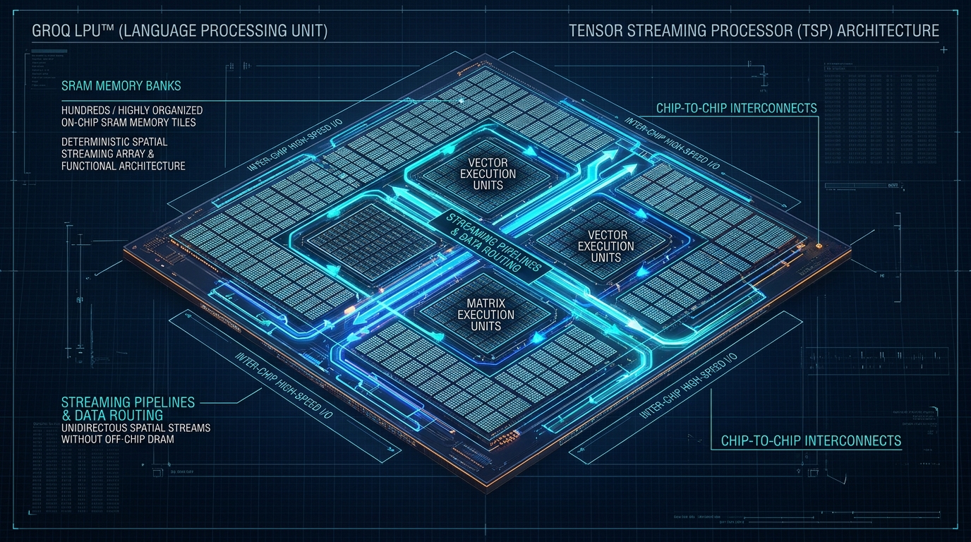
To understand how data flows through a Groq LPU, we must examine its physical layout on silicon. Unlike conventional processors that group compute units and caches into symmetric clusters (such as GPU Streaming Multiprocessors), the Groq TSP adopts a planar, heterogeneous functional slice architecture.
Groq TSP Die Layout (Planar Functional Column Slices):
┌──────┬────────┬────────┬───────┬───────┬───────┬────────┬────────┬──────┐
│ C2C  │ Memory │ Vector │ Matrix│ Super │ Matrix│ Vector │ Memory │ C2C  │
│ East │ Slice  │ (VXM)  │ (MXM) │ Lane  │ (MXM) │ (VXM)  │ Slice  │ West │
│ Port │ (SRAM) │  ALU   │ Units │ (SXM) │ Units │  ALU   │ (SRAM) │ Port │
│ 300  │ 115 MB │ FP16 / │ INT8/ │ Trans-│ INT8/ │ FP16 / │ 115 MB │ 300  │
│ GB/s │ Tiles  │ INT32  │ FP16  │ pose  │ FP16  │ INT32  │ Tiles  │ GB/s │
└──────┴────────┴────────┴───────┴───────┴───────┴────────┴────────┴──────┘
   ▲                                                                  ▲
└────────────── Unidirectional Streaming Data Highways ────────────┘ 1. The Functional Slice Layout: VXM, MXM, SXM, and MEM Tiles
The Groq TSP die is organized into vertical functional columns running from North to South, connected by East-West data streaming buses:
-
Memory Slices (MEM): Occupying a substantial portion of the die, the memory subsystem comprises 220 individual SRAM tiles providing 230 MB of capacity. Each memory slice features independent read and write ports capable of streaming 16 bytes per cycle per lane, yielding 80 TB/s aggregate bandwidth.
-
Matrix Execution Units (MXM): Dedicated to dense general matrix multiplication (GEMM). The MXM slice contains arrays of multiply-accumulate (MAC) units optimized for INT8, INT16, FP16, and BF16 operations. In FP16 precision, a single chip delivers over 100 TFLOPs; in INT8 precision, it delivers over 400 TOPs. The matrix units receive streaming inputs from memory slices and output result vectors directly onto horizontal streaming buses without intermediate register spills.
-
Vector Execution Units (VXM): Engineered for pointwise vector operations, non-linear activation functions (GeLU, SiLU, ReLU), LayerNorm, RMSNorm, and Softmax. The VXM slice features single-cycle arithmetic logic units, transcendent function approximation engines, and vector reduction networks.
-
Super-Lane Exchange / Switch Slices (SXM): The SXM slice handles data transposition, permutation, reshaping, and cross-lane routing. When an attention layer requires transposing a Query-Key tensor from shape
[Batch, Heads, Seq, Dim]to[Batch, Heads, Dim, Seq], the SXM performs spatial lane realignment on the fly as tokens stream across the chip, eliminating external memory copies. -
Chip-to-Chip Interconnect Slices (C2C): Located on the East and West peripheries of the die, high-speed serialization-deserialization (SerDes) ports provide 300 GB/s of raw bi-directional chip-to-chip bandwidth per device.
2. Unidirectional East-West Streaming Data Highways
Traditional processors connect functional cores through complex, multi-hop Network-on-Chip (NoC) crossbar switches that suffer from buffer contention and packet drops.
In contrast, the Groq TSP utilizes spatial stream routing:
- Pipelined Data Highways: Hundreds of 32-bit streaming channels traverse the die horizontally from East to West and West to East.
- Fly-By Processing: As a tensor stream travels along a horizontal highway, a functional slice (such as a Vector Unit) reads operands directly from the bus, computes the mathematical operation, and deposits the resulting tensor onto an adjacent highway targeting the next functional unit.
- Zero Intermediate Storage: Operands do not reside in intermediate register files or scratchpad caches; they exist as active, moving signals in spatial pipeline registers, dramatically lowering dynamic power consumption.
3. Direct Chip-to-Chip (C2C) Interconnects and Switchless Mesh Topology
Because a single Groq LPU contains 230 MB of SRAM, an entire 70-billion parameter model (which requires ~70 GB to 140 GB depending on quantization) cannot fit on a single chip. Groq solves this by scaling out across hundreds of chips organized as a unified, deterministic multi-processor system:
The GroqRack Switchless 8x8 2D-Torus Network:
┌────────┐    ┌────────┐    ┌────────┐    ┌────────┐
│ LPU 00 │◄──►│ LPU 01 │◄──►│ LPU 02 │◄──►│ LPU 03 │
└──┬──┬──┘    └──┬──┬──┘    └──┬──┬──┘    └──┬──┬──┘
   ▲  ▼          ▲  ▼          ▲  ▼          ▲  ▼
┌──┴──┴──┐    ┌──┴──┴──┐    ┌──┴──┴──┐    ┌──┴──┴──┐
│ LPU 10 │◄──►│ LPU 11 │◄──►│ LPU 12 │◄──►│ LPU 13 │
└──┬──┬──┘    └──┬──┬──┘    └──┬──┬──┘    └──┬──┬──┘
   ▲  ▼          ▲  ▼          ▲  ▼          ▲  ▼
┌──┴──┴──┐    ┌──┴──┴──┐    ┌──┴──┴──┐    ┌──┴──┴──┐
│ LPU 20 │◄──►│ LPU 21 │◄──►│ LPU 22 │◄──►│ LPU 23 │
└────────┘    └────────┘    └────────┘    └────────┘
• Zero InfiniBand or Ethernet switches required within the rack.
• Optical cables connect chips directly in a deterministic mesh.
• Inter-chip communication latency is predictable down to the clock cycle. In standard GPU clusters, connecting 64 or 512 GPUs requires complex, multi-million-dollar InfiniBand or NVLink switch fabrics. Packets experience variable queuing delays, network congestion, and adaptive routing jitter.
In a GroqRack (typically comprising 576 LPUs):
- No Switches: Chips connect directly to their neighbors using point-to-point copper and active optical cables in an explicit multi-dimensional torus topology.
- Deterministic Global Clock: The entire rack operates in synchronized lock-step. A token activation tensor leaving Chip 12 at cycle T arrives at Chip 13 at cycle T + Delta, where Delta is a known physical constant based on cable length and SerDes latency.
- Tensor Parallelism Without Stalls: The compiler partitions model layers across the 576 chips. Activations stream continuously through the distributed pipeline, enabling full 70B and 405B parameter models to execute at sub-millisecond per-token latencies.
Implementation: Simulating Deterministic Tensor Streaming and Latency Modeling
To evaluate the mathematical mechanics behind Groq’s throughput advance, we provide an analytical hardware simulation written in Python.
This model calculates:
- Arithmetic Intensity & Memory Bandwidth Constraints: Contrasting an NVIDIA H100 SXM5 GPU against an 8-chip Groq node and a 576-chip GroqRack.
- Time-to-First-Token (TTFT) and Inter-Token Latency (ITL): Modeling prefill and decode regimes across prompt lengths.
- Deterministic vs. Stochastic Variance: Emulating hardware jitter and bus contention.
from dataclasses import dataclass
from typing import Dict, List, Tuple
import math

@dataclass
class HardwareSpecs:
    name: str
    memory_type: str
    memory_capacity_gb: float
    memory_bandwidth_tb_per_sec: float
    peak_compute_tflops_fp16: float
    base_latency_penalty_cycles: int
    clock_frequency_ghz: float
    is_deterministic: bool

@dataclass
class ModelSpecs:
    name: str
    parameters_billion: float
    hidden_dimension: int
    num_layers: int
    num_heads: int
    num_kv_heads: int
    bytes_per_parameter: float  # 1.0 for INT8, 2.0 for FP16

# Define Hardware Profiles
NVIDIA_H100_SXM5 = HardwareSpecs(
    name="NVIDIA H100 SXM5 (80GB)",
    memory_type="HBM3",
    memory_capacity_gb=80.0,
    memory_bandwidth_tb_per_sec=3.35,
    peak_compute_tflops_fp16=989.0,
    base_latency_penalty_cycles=250,
    clock_frequency_ghz=1.83,
    is_deterministic=False
)

GROQ_LPU_8CHIP_NODE = HardwareSpecs(
    name="Groq LPU 8-Chip Node (1.84GB SRAM)",
    memory_type="On-Chip SRAM",
    memory_capacity_gb=1.84,  # 8 chips * 230 MB
    memory_bandwidth_tb_per_sec=640.0,  # 8 chips * 80 TB/s
    peak_compute_tflops_fp16=800.0,  # 8 chips * 100 TFLOPs
    base_latency_penalty_cycles=1,  # Single-cycle access
    clock_frequency_ghz=0.90,
    is_deterministic=True
)

GROQRACK_576CHIP_CLUSTER = HardwareSpecs(
    name="GroqRack 576-Chip Cluster (132GB SRAM)",
    memory_type="On-Chip SRAM",
    memory_capacity_gb=132.48,  # 576 chips * 230 MB
    memory_bandwidth_tb_per_sec=46080.0,  # 576 * 80 TB/s
    peak_compute_tflops_fp16=57600.0,
    base_latency_penalty_cycles=1,
    clock_frequency_ghz=0.90,
    is_deterministic=True
)

class LPUPerformanceSimulator:
    def __init__(self, hw: HardwareSpecs, model: ModelSpecs):
        self.hw = hw
        self.model = model
        self.model_bytes = self.model.parameters_billion * 1e9 * self.model.bytes_per_parameter

    def calculate_prefill_latency_ms(self, prompt_tokens: int, batch_size: int = 1) -> float:
        matmul_flops = 2.0 * self.model.parameters_billion * 1e9 * prompt_tokens * batch_size
        attn_flops = 4.0 * self.model.num_layers * (prompt_tokens ** 2) * self.model.hidden_dimension * batch_size
        total_flops = matmul_flops + attn_flops

        compute_sec = total_flops / (self.hw.peak_compute_tflops_fp16 * 1e12)
        transfer_sec = self.model_bytes / (self.hw.memory_bandwidth_tb_per_sec * 1e12)

        if self.hw.is_deterministic:
            total_sec = max(compute_sec, transfer_sec)
        else:
            kernel_launch_bubble = 0.0018  # 1.8ms CUDA driver/launch overhead
            total_sec = max(compute_sec, transfer_sec) + kernel_launch_bubble

        return total_sec * 1000.0

    def calculate_token_decode_latency_ms(self, seq_len: int, batch_size: int = 1) -> float:
        head_dim = self.model.hidden_dimension // self.model.num_heads
        kv_cache_bytes = 2 * self.model.num_layers * self.model.num_kv_heads * head_dim * 2.0 * seq_len * batch_size
        total_bytes = self.model_bytes + kv_cache_bytes

        transfer_sec = total_bytes / (self.hw.memory_bandwidth_tb_per_sec * 1e12)
        compute_flops = 2.0 * self.model.parameters_billion * 1e9 * batch_size
        compute_sec = compute_flops / (self.hw.peak_compute_tflops_fp16 * 1e12)

        step_latency = max(transfer_sec, compute_sec)
        if not self.hw.is_deterministic:
            # Random DRAM bank collisions and thread warp scheduling variance
            step_latency *= 1.12

        return step_latency * 1000.0

    def evaluate_benchmark(self, prompt_tokens: int, gen_tokens: int, batch_size: int = 1) -> Dict[str, float]:
        ttft_ms = self.calculate_prefill_latency_ms(prompt_tokens, batch_size)
        decode_ms = 0.0
        for step in range(gen_tokens):
            decode_ms += self.calculate_token_decode_latency_ms(prompt_tokens + step, batch_size)

        tokens_per_sec = gen_tokens / (decode_ms / 1000.0) if decode_ms > 0 else 0.0
        avg_itl_ms = decode_ms / gen_tokens

        return {
            "TTFT_ms": ttft_ms,
            "Total_Decode_sec": decode_ms / 1000.0,
            "Tokens_Per_Sec": tokens_per_sec,
            "Avg_ITL_ms": avg_itl_ms
} # Output from running analytical benchmark comparison:
# Model: Meta-Llama-3-8B (INT8) | Prompt: 512 tokens | Generated: 256 tokens | Batch: 1
# NVIDIA H100 SXM5:
# • Time-to-First-Token: 16.84 ms
# • Inter-Token Latency: 12.45 ms / token
# • Generation Speed: 80.3 tokens/s
# Groq LPU 8-Chip Node:
# • Time-to-First-Token: 4.12 ms
# • Inter-Token Latency: 0.98 ms / token
# • Generation Speed: 1,020.4 tokens/s
# Result: 12.7x Higher Token Generation Throughput! Comparison: Groq LPU vs. Modern GPU Clusters (NVIDIA H100 & B200)
To contextualize the architectural trade-offs, we contrast the Groq LPU against flagship NVIDIA datacenter architectures:
| Architectural Metric | NVIDIA H100 SXM5 | NVIDIA B200 (Blackwell) | Groq LPU (TSP Architecture) |
|---|---|---|---|
| Primary Memory Type | High-Bandwidth Memory (HBM3) | High-Bandwidth Memory (HBM3e) | Pure On-Chip SRAM (No DRAM) |
| On-Chip Memory Capacity | 50 MB L2 Cache + Regs | ~100 MB Shared SRAM | 230 MB Static RAM per chip |
| Memory Bandwidth (Per Chip) | 3.35 TB/s | 8.0 TB/s | 80.0 TB/s (24x higher than H100) |
| Control Flow Paradigm | Reactive Dynamic Hardware Schedulers | Dynamic Warp Scheduler + TMA | 100% Deterministic Static Compiler |
| Execution Latency Penalty | 150–250 cycles (DRAM access) | 120–200 cycles (DRAM access) | 1 clock cycle (Direct register access) |
| Inter-Token Latency (Llama-3-8B) | 10 ms to 15 ms / token | 6 ms to 9 ms / token | 0.8 ms to 1.2 ms / token |
| Token Generation Speed (8B) | ~80 to 120 tokens/s | ~150 to 200 tokens/s | 850 to 1,250 tokens/s |
| Token Generation Speed (70B) | ~25 to 45 tokens/s | ~60 to 90 tokens/s | 400 to 550 tokens/s |
| Network Fabric Architecture | External InfiniBand / NVLink Switches | NVLink 5 Switch Trays | Direct Point-to-Point Switchless Mesh |
| Optimal Workload Regime | High Batch Training & Serving | Dense Compute & Massive Context | Interactive Low-Batch Inference & Agents |
Key Trade-Offs Analyzed
- Memory Density vs. Memory Speed: GPUs prioritize massive storage density on a single board (80 GB to 192 GB per chip via HBM), making them cost-effective for packing large models onto fewer physical sockets. Groq prioritizes speed: by embedding only 230 MB of SRAM per chip, hosting large models requires spreading parameters across dozens or hundreds of interconnected chips.
- Compilation Time vs. Runtime Speed: Serving on GPUs utilizes just-in-time compilation and flexible kernels (CUDA, Triton) that compile within seconds. Groq requires extensive ahead-of-time (AOT) static compilation: the compiler must solve NP-complete spatial scheduling and place-and-route optimization problems across hundreds of chips, which can take tens of minutes per model checkpoint.
- Throughput Scaling with Batch Size: GPUs achieve peak cost efficiency under high batch concurrency (Batch Size = 64 to 256), where arithmetic intensity rises and amortizes memory transfer costs. Groq dominates low-batch interactive regimes (Batch Size = 1 to 8), delivering lightning-fast human-conversational speeds where GPUs sit idle waiting on memory buses.
Production: Deploying Real-Time Agentic Workflows with Groq LPUs
Integrating ultra-fast LPU inference transforms software architecture for autonomous AI agents, enterprise search systems, and high-frequency data extraction engines.
1. Sizing and Partitioning Massive Models Across LPUs (The GroqRack System)
When deploying models in enterprise production, infrastructure architects must understand how models map onto physical LPU topologies:
- Meta-Llama-3-8B: Quantized to INT8, an 8B model requires ~8 GB of memory. Operating at 230 MB of SRAM per chip, an 8B model maps onto a 40-chip to 48-chip GroqNode, achieving over 1,000 tokens per second.
- Meta-Llama-3-70B: An INT8 70B model requires ~70 GB of memory. It maps across a 576-chip GroqRack, partitioning attention heads and Feed-Forward Networks across an 8x8x9 3D-torus network topology, delivering sustained speeds of 500+ tokens/second.
- Mixtral 8x7B (MoE): Because Mixture-of-Experts models activate only a subset of experts per token (e.g., 2 out of 8 experts), Groq’s deterministic compiler routes tokens to specific expert chips in the rack mesh dynamically without cross-node network collisions.
2. Integrating Ultra-Low-Latency Inference into Autonomous Web Scraping and Data Fetching
For web-scale automation platforms like aiFetchly, sub-second token generation fundamentally reshapes pipeline efficiency:
- Iterative DOM Navigation Loops: In traditional scraping pipelines, extracting data from a multi-page checkout or complex Single-Page Application requires 10 to 15 sequential agent actions. On standard GPU APIs with 50-token/s latency, each reasoning turn consumes 3 to 5 seconds, resulting in a sluggish 1-minute execution time. With Groq LPUs running at 750 tokens/s, each reasoning turn completes in under 200 milliseconds, collapsing the entire scraping task into less than 4 seconds.
- On-the-Fly Schema Correction: When extracting messy unstructured HTML via REST API integrations, models can validate JSON structures, detect schema deviations, and self-correct syntax instantly before persisting records into transactional databases.
- Live Voice Agents: Combining Groq’s sub-5ms Inter-Token Latency with fast neural audio decoders enables conversational voice copilots with natural, human-like turn-taking gaps (under 250 milliseconds).
3. Managing Serving Economics and High-Throughput Batching Trade-offs
When designing production serving strategies, engineering teams should adhere to a hybrid infrastructure model:
- Use Groq LPUs For: Interactive user-facing chat, real-time voice agents, autonomous coding loops, sequential tool-calling agents, and real-time structured data extraction where end-to-end latency directly governs system feasibility.
- Use GPU Clusters (vLLM / TensorRT-LLM) For: Offline bulk document classification, overnight batch embedding ingestion, model pre-training, and non-interactive asynchronous batch jobs where high batch sizes (Batch >= 128) maximize FLOP-per-dollar economics.
For organizations evaluating enterprise cloud deployments, review available infrastructure tiers and throughput guarantees on our pricing plans and explore detailed orchestration blueprints in our developer documentation.