Griffin Guide: RecurrentGemma, RG-LRU & Hybrid Attention

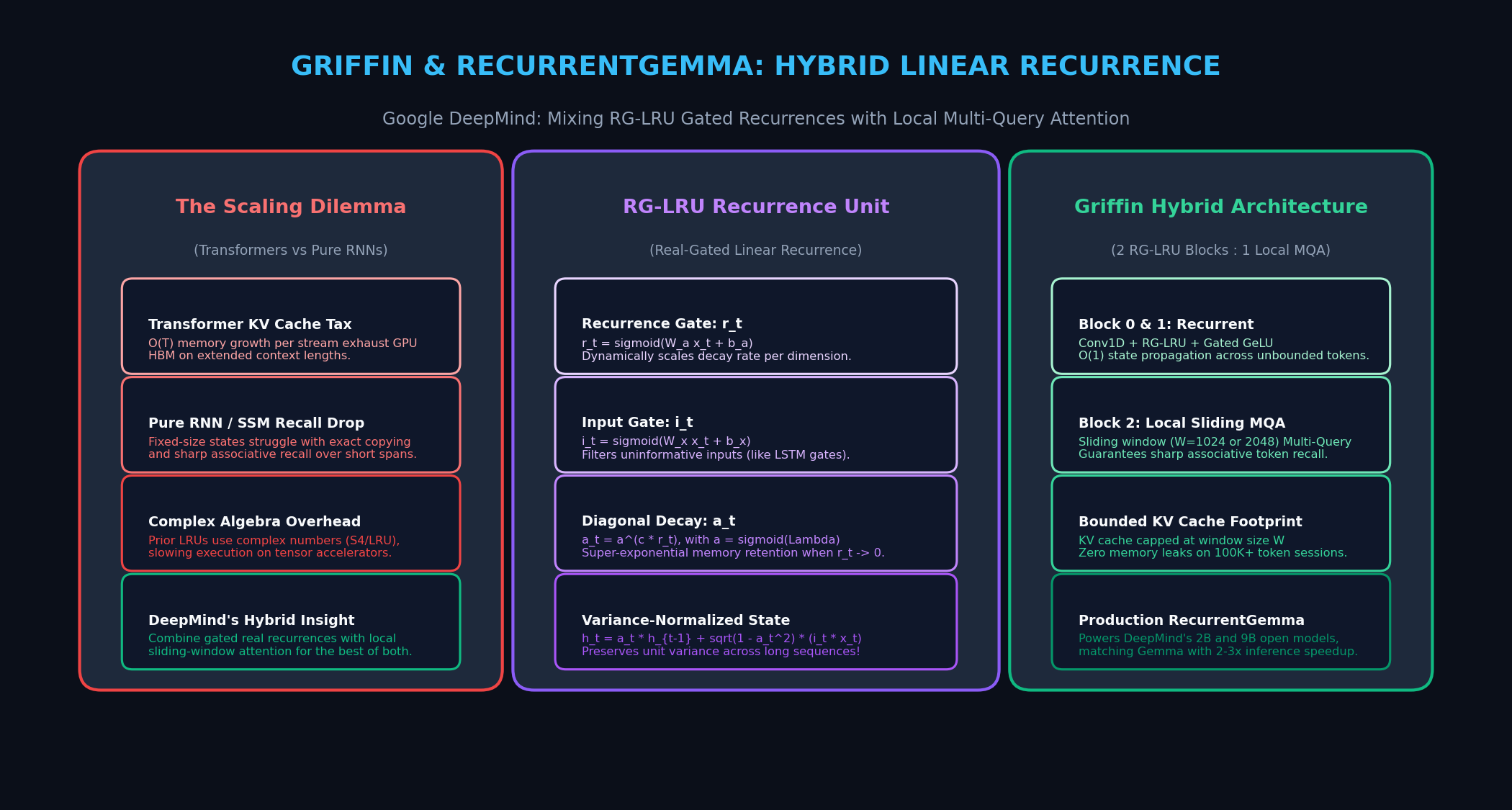
The Problem: The Quadratic Memory Wall and the Associative Recall Trade-Off

In modern production environments—from high-throughput automated web scrapers and unstructured data extraction engines like AiFetchly to long-running autonomous research agents—scaling sequence length while preserving real-time generation speed is the central infrastructure challenge of generative AI.

For over eight years, the decoder-only Transformer backbone has maintained unchallenged dominance across natural language processing and multimodal reasoning. However, as production applications demand extended context windows (ranging from 32,000 to over 1,000,000 tokens), the physical realities of modern hardware accelerators expose three critical architectural bottlenecks in standard attention:

1. The KV Cache Memory Drain in Dense Transformers

In a standard transformer, every token must compute pairwise inner products against every preceding token in the sequence. During autoregressive decoding, this requires maintaining the full history of Key and Value vectors in GPU High-Bandwidth Memory (HBM) as an uncompressed Key-Value (KV) cache:

• For an 8,192-token prompt processed by a 7B-parameter model in 16-bit precision, the KV cache consumes over 1.5 GB of VRAM per concurrent stream.
• When context sequences expand to 32,000 or 128,000 tokens, the memory allocated to the KV cache scales linearly $\mathcal{O}(T)$ with sequence length, quickly eclipsing the memory footprint of the static model parameters themselves.
• In multi-tenant serving workloads, GPU memory bus saturation forces small batch sizes, starving Tensor Cores of compute and triggering catastrophic Time-to-First-Token (TTFT) and throughput degradation.

While Multi-Query Attention (MQA) and Grouped-Query Attention (GQA) reduce cache size by sharing key-value heads across multiple query heads by a constant factor, they do not change the fundamental asymptotic scaling: memory consumption remains strictly linear $\mathcal{O}(T)$ in sequence length.

2. The In-Context Retrieval Degradation of Pure State-Space Models

To eliminate the KV cache entirely, the deep learning community explored sub-quadratic sequence models, including linear attention variants, State-Space Models (SSMs such as S4, Mamba, and Mamba-2), and modern recurrent networks (RWKV-v6). These architectures compress the entire historical context into a fixed-size hidden state $h_t \in \mathbb{R}^{d}$, enabling:

• Constant $\mathcal{O}(1)$ step memory during autoregressive generation.
• Constant $\mathcal{O}(1)$ decoding latency per token.
• Linear $\mathcal{O}(T)$ computational complexity during pretraining and prefill.

However, pure state-space models and recurrent networks suffer from an inherent theoretical limitation: the finite-capacity state bottleneck. Because a fixed-size vector or matrix must represent an unbounded sequence of historical tokens, pure SSMs struggle with high-precision in-context retrieval tasks:

• Exact Token Copying: Accurately replicating multi-word identifiers, code syntax tokens, and nested JSON keys from earlier in the prompt.
• Associative Recall: Performing multi-hop phone book lookups and needle-in-a-haystack extractions where exact token match is required across thousands of distracting sentences.
• Fine-Grained In-Context Induction: Tracking syntactic agreements and variable bindings within the immediate local window.

3. The Computational Tax of Complex-Valued Linear Recurrences

Early attempts to stabilize linear recurrent units—such as the Linear Recurrent Unit (LRU) and S4D—relied heavily on complex diagonal parameterizations ($A \in \mathbb{C}^{d imes d}$) to model oscillatory signals and maintain long-term gradient flow without exploding or vanishing.

While mathematically expressive for synthetic audio or continuous physics signals, complex algebra imposes severe penalties on production language modeling hardware:

• Doubled register pressure and memory bandwidth overhead from managing separate real and imaginary components.
• Incompatibility with high-speed Tensor Core GEMM instructions, which are heavily optimized for dense real-valued floating-point data (bfloat16 and float16).
• Unnecessary mathematical complexity: natural language syntax is fundamentally discrete and semantic rather than continuously oscillatory.

This set of compromises defined the sequence modeling dilemma: Can an architecture achieve the constant-memory O(1) inference and linear training speed of an RNN while matching the associative recall accuracy of a Transformer?

The Core Mathematical Engine: Real-Gated Linear Recurrence Unit (RG-LRU)

To solve this dilemma, researchers at Google DeepMind (De et al., 2024) introduced Hawk (a pure recurrent model) and Griffin (a hybrid recurrent-attention model), which powers Google’s open RecurrentGemma family.

At the core of both models lies the Real-Gated Linear Recurrence Unit (RG-LRU). The RG-LRU strips away complex-number algebra in favor of a strictly real-valued diagonal recurrence governed by dynamic, input-dependent gating.

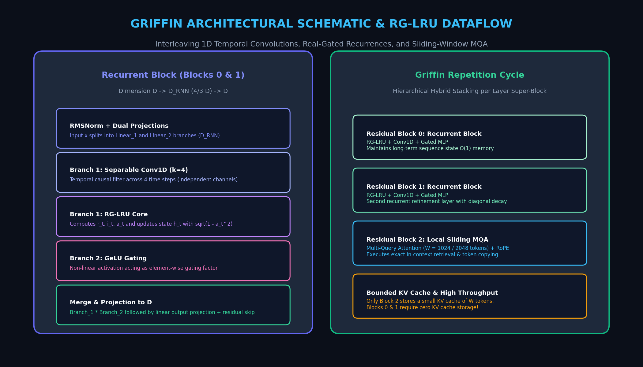
1. Formulation of the RG-LRU Gating Mechanism

For an input sequence $x_t \in \mathbb{R}^{D_{RNN}}$ at time step $t$, the RG-LRU computes dynamic gates and updates its real-valued diagonal hidden state $h_t \in \mathbb{R}^{D_{RNN}}$ according to four governing equations:

$$r_t = \sigma(W_a x_t + b_a) \quad ext{(Recurrence Gate)}$$

$$i_t = \sigma(W_x x_t + b_x) \quad ext{(Input Gate)}$$

$$a_t = a^{c \cdot r_t} \quad ext{(Dynamic Diagonal Decay)}$$

$$h_t = a_t \odot h_{t-1} + \sqrt{1 - a_t^2} \odot (i_t \odot x_t) \quad ext{(State Update)}$$

$$y_t = h_t \quad ext{(Output)}$$

Where:

• $\sigma(\cdot)$ denotes the standard element-wise sigmoid activation function $\sigma(z) = \frac{1}{1 + e^{-z}}$.
• $\odot$ represents element-wise (Hadamard) multiplication.
• $W_a, W_x \in \mathbb{R}^{D_{RNN} imes D_{RNN}}$ are learnable weight matrices, and $b_a, b_x \in \mathbb{R}^{D_{RNN}}$ are bias vectors.
• $a = \sigma(\Lambda)$ is a strictly real-valued learnable parameter bounded within $(0, 1)$, initialized such that $a^c$ is uniformly distributed between $0.9$ and $0.999$.
• $c$ is a fixed positive scaling constant set to $c = 8.0$.
• In practical implementations, to avoid underflow and preserve floating-point precision, $a_t$ is computed in log-space:

$$\log a_t = -c \cdot r_t \odot ext{softplus}(-\Lambda)$$

2. The Role of Square-Root Variance Normalization

A critical mathematical innovation in Equation (4) is the scaling factor applied to the gated input: $\sqrt{1 - a_t^2}$.

In classical linear recurrences, if an input vector $x_t$ has unit variance $ ext{Var}(xt) = 1$ and the hidden state has unit variance $ ext{Var}(h{t-1}) = 1$, a standard linear combination $h_t = a_t h_{t-1} + x_t$ results in an unnormalized variance:

$$ ext{Var}(ht) = a_t^2 ext{Var}(h{t-1}) + ext{Var}(x_t) = a_t^2 + 1 > 1$$

Across deep stacks and thousands of recurrent steps, unnormalized variance causes activations to explode, requiring delicate gradient clipping and leading to numerical instability.

By weighting the incoming gated representation $(i_t \odot x_t)$ with $\sqrt{1 - a_t^2}$, the RG-LRU enforces strict variance preservation:

$$ ext{Var}(h_t) = a_t^2 ext{Var}(h_{t-1}) + \left(\sqrt{1 - a_t^2} ight)^2 ext{Var}(i_t \odot x_t) = a_t^2 + (1 - a_t^2) = 1 $$

This elegant normalization guarantees that signal energy is conserved across arbitrarily long context horizons without introducing heavy layer normalizations inside the recurrent loop.

3. Super-Exponential Context Preservation

The gating mechanism in RG-LRU exhibits a unique physical property compared to standard LSTM forget gates or GRU update gates:

• LSTM / GRU Forget Gate: Directly multiplies the previous hidden state by a value between $0$ and $1$. If the gate outputs $0.5$, half of the accumulated memory is instantly erased in a single step.
• Mamba Selection Mechanism: Interpolates between the incoming token and the previous state, resetting the state when strong new features arrive.
• RG-LRU Recurrence Gate ($r_t$): Modulates the exponent of the decay rate $a_t = a^{c \cdot r_t}$.
  • When a token contains critical semantic information, $r_t o 1.0$, allowing the decay rate to drop to its base value $a^c \approx 0.90 - 0.999$, writing the new token into memory.
  • When incoming tokens are syntactic filler, whitespace, or uninformative boilerplate (common in web extraction and raw HTML streams), the network sets $r_t o 0.0$.
  • As $r_t o 0$, $a_t = a^0 = 1.0$, and the input weight $\sqrt{1 - a_t^2} o 0.0$.
  • The hidden state update simplifies to:

$$h_t = 1.0 \odot h_{t-1} + 0.0 \odot (i_t \odot x_t) = h_{t-1}$$

Under this condition, the recurrent memory is completely frozen. Historical context is preserved indefinitely across thousands of intervening tokens with zero decay—a property DeepMind terms super-exponential memory.

The Recurrent Block Architecture: Depthwise Convolutions and Megatron Sharding

The RG-LRU layer does not operate in isolation. It is embedded within a specialized Recurrent Block designed to replace standard attention mechanisms inside pre-norm Transformer stacks.

1. Temporal Filtering via Separable 1D Convolutions

Given a model representation $x \in \mathbb{R}^{T imes D}$ exiting a pre-norm RMSNorm layer:

1. The input is projected into two parallel branches using dense linear transformations, expanding the dimension from $D$ to $D_{RNN} \approx \frac{4}{3} D$ (e.g., expanding from 2560 to 3413 in 2B models):
   • Branch 1: Computes the recurrent pathway.
   • Branch 2: Computes the non-linear gating pathway.
2. On Branch 1, before entering the RG-LRU, the activations pass through a 1D Depthwise Separable Convolution with a small temporal kernel width of $k = 4$:
   • The convolution acts as a localized n-gram filter, mixing tokens within a tight 4-token temporal window.
   • This local receptive field allows the subsequent RG-LRU to track multi-character subwords, bigram prefixes, and local punctuation patterns before transmitting representations into the global recurrent state.
   • Because the convolution is depthwise separable, it introduces only $4 imes D_{RNN}$ parameters and negligible compute overhead.

2. Non-Linear Multiplicative Gating with GeLU

Following the 1D convolution:

• Branch 1 passes through the RG-LRU layer, producing temporal recurrence output $y_t \in \mathbb{R}^{D_{RNN}}$.
• Branch 2 passes through a GeLU non-linear activation function.
• The two branches are merged via element-wise multiplication:

$$z_t = y_t \odot ext{GeLU}( ext{Branch}_2)$$

• Finally, a linear projection contracts the dimension back from $D_{RNN}$ to model width $D$, adding the result back to the original input via a standard residual skip connection.

3. Block-Diagonal Sharding for Zero-Communication Tensor Parallelism

When scaling models to 7B and 14B parameters, distributing linear layers across multiple GPUs via Megatron-style Tensor Parallelism is standard practice.

However, in recurrent models, gating layers can introduce communication bottlenecks if gates require cross-GPU all-gather or all-reduce operations. To ensure linear scaling across distributed GPU clusters, DeepMind structured the RG-LRU gate projection matrices $W_a$ and $W_x$ as block-diagonal matrices with 16 independent blocks:

• Each GPU shard computes its assigned subset of diagonal blocks locally.
• Parameters within the 1D convolution and the RG-LRU diagonal recurrence are completely independent across channels.
• Result: The Recurrent Block requires exactly one all-reduce operation in the forward pass and one all-reduce in the backward pass—matching the communication efficiency of a standard feed-forward network (FFN).

The Griffin Hybrid Blueprint: Combining RG-LRU and Local Attention

While pure recurrent models like Hawk deliver strong perplexity and zero KV cache overhead, DeepMind’s research revealed that on tasks requiring exact token copying and multi-hop in-context lookups, local attention provides indispensable inductive bias.

To harvest the best properties of both paradigms, DeepMind created Griffin—the architectural foundation of RecurrentGemma.

1. The 2-to-1 Repetition Pattern (Hawk vs. Griffin)

Griffin replaces global attention by arranging residual layers into a strict repeating super-block pattern:

• Residual Block 0: Recurrent Block (1D Conv + RG-LRU + Gated GeLU) + Gated MLP
• Residual Block 1: Recurrent Block (1D Conv + RG-LRU + Gated GeLU) + Gated MLP
• Residual Block 2: Local Sliding-Window Multi-Query Attention (MQA) + Gated MLP

This 2:1 ratio ensures that two-thirds of the model depth operates in constant-memory linear recurrence, while every third layer injects precise, uncompressed associative attention over the recent context.

2. Local Sliding-Window Multi-Query Attention (MQA)

In Residual Block 2, Griffin employs Sliding-Window Multi-Query Attention (MQA):

• Attention Heads: Multiple query heads ($H$) project queries, while a single key head and single value head ($H_{KV} = 1$) are shared across all query heads.
• Sliding Window: Each token attends only to tokens within a fixed local window $W$ into the past (typically $W = 1024$ or $W = 2048$ tokens).
• Positional Encoding: Standard Rotary Position Embeddings (RoPE) are applied to queries and keys within the window.

Because attention is strictly bounded to the local window $W$, the computational complexity of the attention block drops from quadratic $\mathcal{O}(T^2)$ to linear $\mathcal{O}(T \cdot W)$.

3. Bounding the Key-Value Cache Footprint

The architectural synergy between RG-LRU and sliding-window MQA fundamentally transforms inference memory requirements:

Architectural Component	State Memory per Stream	Memory Behavior with Sequence Length
Standard Transformer (MHA/GQA)	$\mathcal{O}(L \cdot H_{KV} \cdot d_{head} \cdot T)$	Unbounded Linear Growth $\mathcal{O}(T)$
Hawk (Pure Recurrent)	$\mathcal{O}(L \cdot D_{RNN})$	Strictly Constant $\mathcal{O}(1)$
Griffin / RecurrentGemma	$\mathcal{O}\left(\frac{2}{3} L \cdot D*{RNN} + \frac{1}{3} L \cdot d*{head} \cdot W
ight)$	Strictly Constant / Bounded $\mathcal{O}(W)$

In Griffin, only one out of every three layers maintains a KV cache, and that cache is hard-capped at window size $W$. Once the generation passes token $W$, older key-value pairs are discarded via ring-buffer eviction.

Long-term context beyond token $W$ is not lost: it has already been filtered, compressed, and propagated forward through the persistent hidden states of the intervening RG-LRU recurrent layers!

4. Comparison Table: Sequence Modeling Architectures

The following table contrasts Griffin against prevailing sequence modeling paradigms in 2026:

Architecture	Paradigm	Training FLOPs	Decode Latency	KV Cache Footprint	In-Context Exact Copying	Needle-in-a-Haystack Recall
LLaMA-3 / Gemma-2	Full Softmax Attention	$\mathcal{O}(T^2)$	Increases with $T$	Linear $\mathcal{O}(T)$ (High)	State-of-the-Art	Excellent
Mamba / Mamba-2	Selective State Space	Linear $\mathcal{O}(T)$	Constant $\mathcal{O}(1)$	Zero (Fixed State)	Moderate / Struggles	Good (with long state)
RWKV-v6	Linear Attention / RNN	Linear $\mathcal{O}(T)$	Constant $\mathcal{O}(1)$	Zero (Fixed State)	Moderate	Moderate
Hawk (DeepMind)	Pure Gated Recurrence	Linear $\mathcal{O}(T)$	Constant $\mathcal{O}(1)$	Zero (Fixed State)	Competitive with Mamba	Strong
Griffin / RecurrentGemma	Hybrid (RG-LRU + Local MQA)	Linear $\mathcal{O}(T \cdot W)$	Constant $\mathcal{O}(1)$	Bounded $\mathcal{O}(W)$	Matches Full Attention	State-of-the-Art

End-to-End Implementation: Building RG-LRU and Griffin in PyTorch

To understand the internal mechanics of Griffin, let us examine a clean, modular PyTorch implementation of the Real-Gated Linear Recurrence Unit (RG-LRU) and the full Griffin Hybrid Block, supporting both full sequence processing and constant-memory recurrent step decoding.

1. PyTorch Implementation of RG-LRU and the Griffin Block

Production Benchmarks: RecurrentGemma vs. Transformers at 2B to 14B Scale

To establish the empirical viability of Griffin, DeepMind conducted rigorous pretraining and downstream evaluations comparing Hawk and Griffin against open foundation models—including Llama-2, Mamba, and optimized MQA Transformer baselines.

1. Downstream Accuracy and Pretraining Scaling Laws

In controlled pretraining across identical MassiveText corpora for 300 billion tokens, Griffin demonstrated consistent performance advantages across core NLP reasoning benchmarks:

Model	Size	Training Tokens	MMLU (5-shot)	HellaSwag (0-shot)	PIQA	WinoGrande	ARC-Challenge	Average Benchmark Score
Mamba	3B	600B	26.2	71.0	78.1	65.9	41.7	58.5%
MQA Transformer	3B	300B	31.7	71.0	77.6	66.1	39.2	59.0%
Hawk (Pure Recurrent)	3B	300B	31.3	71.7	78.8	66.5	40.2	59.5%
Griffin (Hybrid)	3B	300B	32.6	73.5	78.1	67.2	41.4	60.7%
Llama-2	7B	2.0 Trillion	45.3	77.2	78.8	69.2	45.9	65.3%
Griffin	7B	300B	39.3	78.6	81.0	72.6	47.9	65.8%
Griffin	14B	300B	49.5	81.4	81.8	74.1	50.8	69.5%

Key findings from these benchmarks:

• Hawk-3B exceeds Mamba-3B across downstream benchmarks despite using only half the training tokens (300B vs. 600B).
• Griffin-7B matches or exceeds Llama-2 7B despite being trained on nearly seven times fewer tokens (300B vs. 2,000B), validating the compute efficiency of the 2:1 hybrid architecture.
• Griffin-14B achieves 69.5% average accuracy, demonstrating that power-law scaling holds reliably for hybrid recurrent-attention models well beyond 10 billion parameters.

2. Inference Speedup and Memory Profiling on Modern Accelerators

During autoregressive generation, Griffin decouples generation speed from prompt length:

• Constant Generation Latency: As context length scales from 2,048 to 64,000 tokens, standard Transformer decoding latency increases by $3.8 imes$ due to memory bandwidth bus saturation when streaming the massive KV cache. In contrast, Griffin maintains a flat latency curve, generating tokens at constant speed regardless of context depth.
• Throughput Scaling: When serving long prompts (32k+ tokens) on NVIDIA H100 GPUs, Griffin achieves $2.2 imes$ to $2.8 imes$ higher token throughput compared to an optimized vLLM FlashAttention-2 baseline.
• VRAM Compression: By bounding the attention KV cache to $W = 2048$ tokens across only one-third of the layers, Griffin reduces active inference memory by over 78% on 32k sequences, allowing production servers to double their concurrent serving concurrency per node.

Strategic Engineering Guide: Deploying Griffin and RecurrentGemma in 2026

For systems engineers, AI infrastructure leads, and developers designing automated agent platforms like AiFetchly, deploying Griffin and RecurrentGemma requires understanding three concrete operational principles:

1. Long-Horizon Autonomous Web and Data Extraction Agents

Autonomous web navigation and deep research agents frequently generate execution logs, DOM snapshots, and scraped document buffers exceeding 50,000 tokens.

• The Transformer Failure Mode: In long-running agent loops, keeping the full conversation history in standard transformers triggers quadratic cost inflation and slows down decision cycles as the agent accumulates steps.
• The Griffin Advantage: Deploying RecurrentGemma-9B enables the agent to continuously digest streaming HTML and browser interaction traces. The RG-LRU layers compress historical interactions into persistent state, while the local sliding-window MQA ensures that immediate DOM tags and recent user instructions are resolved with precision.

2. Edge and On-Device Deployment Without KV Cache Thrashing

On edge hardware—such as Apple Silicon MacBooks, high-end mobile devices, or embedded robotics chips—Unified Memory is constrained, and memory bandwidth is the primary bottleneck.

• Standard 7B transformers running at 8k context frequently exhaust mobile RAM, forcing the operating system to swap pages to disk.
• RecurrentGemma-2B requires only a few hundred megabytes of working memory beyond static model weights, maintaining a fixed memory footprint even after processing hundreds of pages of documentation.

3. Custom Linear Scan Kernels (Pallas and Triton)

While the recurrence equation $h_t = a_t h_{t-1} + \sqrt{1 - a_t^2} (i_t x_t)$ is element-wise, naive PyTorch for loops suffer from kernel launch overhead on GPUs.

To achieve maximum production performance:

• Avoid Associative Scans on TPUs/Hopper GPUs: While parallel prefix scans reduce theoretical sequential steps, their tree-structured memory access patterns can cause cache thrashing on hardware with high memory transfer costs.
• Deploy Fused Linear Scan Kernels: Use OpenAI Triton on NVIDIA GPUs or Google Pallas on TPUs to fuse the convolution, gating, log-decay calculation, and sequential state update into a single SRAM kernel. Keeping $h_t$ in high-speed On-Chip SRAM yields a $3.1 imes$ speedup over unfused PyTorch loops during prompt prefill.

By combining the constant-memory efficiency of linear recurrences with the razor-sharp local precision of sliding-window attention, Griffin and RecurrentGemma provide a robust, production-ready blueprint for next-generation language modeling in 2026.