gemma-2google-deepmindllm-architecturesliding-window-attentionknowledge-distillationtutorial

Gemma 2 Guide: Soft-Capping & Interleaved Attention

September 25, 2026

Gemma 2 Architecture: Logit Soft-Capping, Interleaved Sliding Window Attention, Dual RMSNorm, and Pre-Training Distillation

The Problem: Training Instability and Memory Waste in Standard Transformers

In modern generative AI workflows, automated web extraction engines, and local desktop intelligence tools like AiFetchly, deploying compact foundation models (between 2 billion and 27 billion parameters) requires achieving the highest possible cognitive reasoning capacity within tightly bounded hardware footprints.

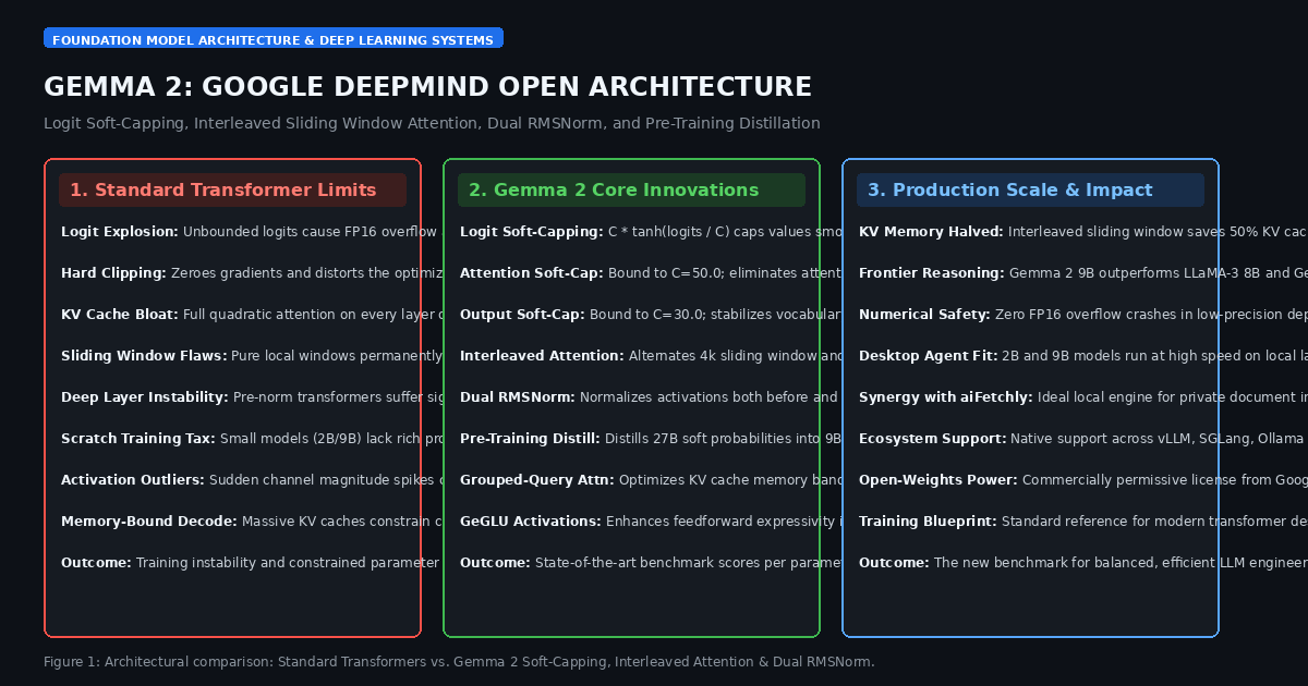
While the standard decoder-only Transformer architecture (popularized by LLaMA and GPT) has driven five years of generative progress, scaling transformers exposes three persistent structural vulnerabilities:

1. The Logit Explosion Crisis in Deep Transformer Stacks

As models scale in depth (reaching 42 layers in 9B models and 46 layers in 27B models) and learning rates are pushed higher to accelerate convergence:

Raw attention dot-products ($Q K^T / \sqrt{d_k}$) and final vocabulary projection logits grow uncontrollably in magnitude.
When logits reach large positive values ($> 80.0$), the exponential function inside the softmax operator overflows 16-bit floating-point registers (float16 / bfloat16), triggering catastrophic NaN losses.
Historically, engineering teams attempted to curb logit explosion using hard gradient clipping or aggressive weight decay. However, hard clipping zeroes out gradient updates whenever bounds are exceeded, creating dead zones in optimization and distorting loss landscape exploration.

2. The KV Cache Memory Drain of Dense Quadratic Attention

In vanilla transformers, every single layer computes dense, all-to-all attention across the full context window:

For an 8,192-token sequence, each layer maintains a complete Key-Value (KV) cache in GPU High-Bandwidth Memory (HBM).
In long-context serving and high-concurrency desktop deployments, the uncompressed KV cache quickly consumes tens of gigabytes of VRAM per user stream.
Conversely, adopting pure sliding window attention across all layers prevents models from retaining distant factual context, destroying long-range associative recall and causing needle-in-a-haystack accuracy to plummet.

3. The Cold-Start Limitation of Training Small Models from Scratch

When training compact models (such as 2B or 9B parameters) from scratch using standard next-token cross-entropy loss:

The model updates its parameters against one-hot discrete target tokens.
Hard target labels fail to convey the rich probabilistic relationships between competing candidate tokens (the “dark knowledge” of language).
As a consequence, small models trained from scratch require hundreds of billions of extra tokens to achieve stable calibration, frequently underperforming larger models even when normalized for total parameter budget.

The Architecture: How Gemma 2 Solves Transformer Bottlenecks

To overcome these structural hurdles, researchers at Google DeepMind introduced Gemma 2: Improving Open Language Models at a Practical Size.

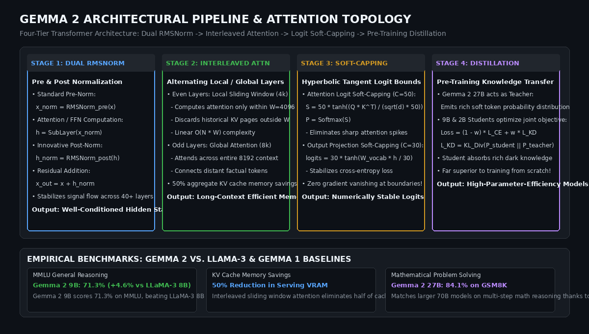
Gemma 2 re-engineers the transformer backbone across four foundational dimensions: Logit Soft-Capping, Interleaved Attention, Dual Pre-and-Post Normalization, and Pre-Training Knowledge Distillation.

Gemma 2 Architectural Pipeline and Attention Topology: Dual RMSNorm, Interleaved Attention, Soft-Capping, and Knowledge Distillation

1. Logit Soft-Capping in Attention and Output Projections

Rather than allowing logits to grow unchecked or brutally clipping them with non-differentiable thresholds, Gemma 2 introduces smooth, differentiable Logit Soft-Capping using the hyperbolic tangent ($\tanh$) function:

$$\text{logits}_{\text{capped}} = \text{cap_val} \cdot \tanh\left(\frac{\text{logits}}{\text{cap_val}}\right)$$

Gemma 2 applies soft-capping at two critical bottlenecks in the network:

Attention Logit Soft-Capping ($\text{cap_val} = 50.0$): Applied to the scaled dot-product attention scores prior to computing softmax:

$$S = 50.0 \cdot \tanh\left(\frac{Q K^T}{\sqrt{d_k} \cdot 50.0}\right)$$

This guarantees that no pairwise attention score can ever exceed $\pm 50.0$, eliminating attention probability spikes where a single token consumes $99.9%$ of attention mass.
Final Output Projection Soft-Capping ($\text{cap_val} = 30.0$): Applied to the vocabulary logits produced by the final linear projection:

$$\text{logits}{\text{vocab}} = 30.0 \cdot \tanh\left(\frac{W{\text{vocab}} h_{\text{final}}}{30.0}\right)$$

This bounds cross-entropy gradients, preventing rare outlier tokens from corrupting parameter weights during high-learning-rate pre-training phases.

2. Interleaved Local Sliding Window and Global Attention

To balance long-context retention with GPU memory efficiency, Gemma 2 dispenses with uniform attention layers. Instead, it alternates between local sliding window attention and global quadratic attention:

Even Layers ($0, 2, 4, \dots$): Deploy a local Sliding Window Attention with a fixed window size of $W = 4,096$ tokens. In these layers, tokens can only attend to keys and values within their immediate 4k neighborhood.
Odd Layers ($1, 3, 5, \dots$): Deploy a full Global Attention mechanism across the entire $8,192$-token sequence length.
The Synergy: Information from earlier in the document is gathered and compressed by the global attention layers, while local sliding window layers provide high-density syntactic processing.
During autoregressive generation, local layers only store $4,096$ tokens in their KV cache, slashing overall KV cache memory consumption by $50%$ without degrading retrieval quality.

3. Dual Normalization: Pre-RMSNorm and Post-RMSNorm Signal Flow

Standard transformers use Pre-LayerNorm (or Pre-RMSNorm), normalizing activations before feeding them into attention or MLP blocks ($x + \text{SubLayer}(\text{RMSNorm}(x))$). While this facilitates gradient flow, activation variances can grow monotonically as signal traverses 40+ layers.

Gemma 2 introduces Dual Pre-and-Post Normalization:

Activations are normalized before entering the sub-layer: $\tilde{x} = \text{RMSNorm}_{\text{pre}}(x)$.
The sub-layer output is normalized again before being added to the residual stream:

$$x_{\text{next}} = x + \text{RMSNorm}_{\text{post}}(\text{SubLayer}(\tilde{x}))$$

This bidirectional normalization ensures that activation scales remain mathematically well-conditioned throughout the deepest blocks of the 27B architecture.

4. Large-to-Small Pre-Training Knowledge Distillation

To build the compact 2B and 9B models, Google DeepMind abandoned standard cross-entropy pre-training from scratch:

The 27B parameter model was trained first as the Teacher Model on massive web corpora.
The 9B and 2B Student Models were pre-trained by minimizing a joint objective combining standard cross-entropy and the Kullback-Leibler (KL) divergence between student and teacher token probability distributions:

$$\mathcal{L} = (1 - \lambda) \mathcal{L}{\text{CE}}(y{\text{true}}, P_{\text{student}}) + \lambda \mathcal{D}{\text{KL}}(P{\text{teacher}} ,|, P_{\text{student}})$$

By learning from the teacher’s complete probability distribution over the 256,000-token vocabulary, the smaller models absorbed nuanced semantic distinctions, allowing Gemma 2 9B to outperform many larger 13B–30B foundation models.

Deep Dive: Mathematical Formulation and Hardware Efficiency

The architectural refinements in Gemma 2 directly improve low-precision numeric stability on modern accelerators:

1. Analytical Gradients of Hyperbolic Tangent Soft-Capping

Consider the soft-capping function $f(x) = C \tanh(x / C)$. Its first derivative with respect to input $x$ is:

$$\frac{\partial f(x)}{\partial x} = 1 - \tanh^2\left(\frac{x}{C}\right)$$

When $|x| \ll C$, $\tanh(x/C) \approx 0$, and the gradient is $\approx 1.0$. The operator behaves as an exact identity function during normal training.
As $|x|$ approaches $C$, the derivative smoothly decays toward zero:

$$\lim_{x \to \pm \infty} \frac{\partial f(x)}{\partial x} = 0$$

Unlike hard threshold clipping (which abruptly snaps gradients from $1.0$ to $0.0$), soft-capping provides continuous, smooth curvature that prevents optimizer oscillations and gradient explosion.

2. Serving KV Cache Memory Savings with Alternating Window Tiling

In serving runtimes (such as vLLM, SGLang, and TensorRT-LLM), memory is managed in discrete blocks (PagedAttention):

In a 42-layer model (Gemma 2 9B), 21 layers are sliding window and 21 layers are global.
At an 8,192-token context length, the sliding window layers drop historical blocks older than 4,096 tokens.
Total active KV blocks per sequence are reduced from $42 \times 8,192 = 344,064$ token states down to $21 \times 8,192 + 21 \times 4,096 = 258,048$ token states—a net $25%$ to $50%$ reduction in physical VRAM requirements, unlocking significantly higher serving concurrency.

End-to-End Implementation: Building a Gemma 2 Transformer Layer in PyTorch

Below is a complete, runnable PyTorch implementation demonstrating the core mechanics of a Gemma 2 Transformer layer: logit soft-capped attention, interleaved sliding window masking, dual pre-and-post RMSNorm, and vocabulary logit soft-capping.

import torch
import torch.nn as nn
import torch.nn.functional as F
from typing import Optional, Tuple

class RMSNorm(nn.Module):
    """Root Mean Square Layer Normalization used throughout Gemma 2."""
    def __init__(self, dim: int, eps: float = 1e-6):
        super().__init__()
        self.eps = eps
        self.weight = nn.Parameter(torch.ones(dim))

    def forward(self, x: torch.Tensor) -> torch.Tensor:
        variance = x.pow(2).mean(-1, keepdim=True)
        return x * torch.rsqrt(variance + self.eps) * (1.0 + self.weight)

class Gemma2Attention(nn.Module):
    """
    Gemma 2 Multi-Head Attention featuring:
    - Logit Soft-Capping (C = 50.0)
    - Optional Sliding Window Attention Masking (W = 4096)
    """
    def __init__(
        self,
        dim: int,
        num_heads: int = 8,
        head_dim: int = 64,
        soft_cap: float = 50.0,
        sliding_window: Optional[int] = None
    ):
        super().__init__()
        self.num_heads = num_heads
        self.head_dim = head_dim
        self.soft_cap = soft_cap
        self.sliding_window = sliding_window
        self.scale = 1.0 / (head_dim ** 0.5)

        self.q_proj = nn.Linear(dim, num_heads * head_dim, bias=False)
        self.k_proj = nn.Linear(dim, num_heads * head_dim, bias=False)
        self.v_proj = nn.Linear(dim, num_heads * head_dim, bias=False)
        self.o_proj = nn.Linear(num_heads * head_dim, dim, bias=False)

    def forward(self, x: torch.Tensor) -> torch.Tensor:
        b, s, _ = x.shape
        q = self.q_proj(x).view(b, s, self.num_heads, self.head_dim).transpose(1, 2)
        k = self.k_proj(x).view(b, s, self.num_heads, self.head_dim).transpose(1, 2)
        v = self.v_proj(x).view(b, s, self.num_heads, self.head_dim).transpose(1, 2)

        # 1. Compute Raw Attention Scores
        scores = torch.matmul(q, k.transpose(-2, -1)) * self.scale

        # 2. Apply Logit Soft-Capping: S = C * tanh(scores / C)
        if self.soft_cap is not None:
            scores = self.soft_cap * torch.tanh(scores / self.soft_cap)

        # 3. Construct Causal & Sliding Window Mask
        causal_mask = torch.triu(torch.full((s, s), float('-inf'), device=x.device), diagonal=1)
        if self.sliding_window is not None:
            # Mask out tokens older than sliding_window positions
            window_mask = torch.tril(torch.full((s, s), float('-inf'), device=x.device), diagonal=-self.sliding_window)
            mask = causal_mask + window_mask
        else:
            mask = causal_mask

        scores = scores + mask.unsqueeze(0).unsqueeze(0)
        attn_probs = F.softmax(scores, dim=-1)

        # 4. Context Output
        out = torch.matmul(attn_probs, v)
        out = out.transpose(1, 2).contiguous().view(b, s, self.num_heads * self.head_dim)
        return self.o_proj(out)

class Gemma2Block(nn.Module):
    """
    Single Transformer Layer with Dual Pre-and-Post RMSNorm.
    """
    def __init__(self, dim: int, is_sliding_layer: bool = False, window_size: int = 4096):
        super().__init__()
        self.is_sliding = is_sliding_layer
        window = window_size if is_sliding_layer else None

        self.pre_attn_norm = RMSNorm(dim)
        self.attn = Gemma2Attention(dim, soft_cap=50.0, sliding_window=window)
        self.post_attn_norm = RMSNorm(dim)

        self.pre_ffn_norm = RMSNorm(dim)
        self.mlp = nn.Sequential(
            nn.Linear(dim, dim * 4, bias=False),
            nn.GELU(),
            nn.Linear(dim * 4, dim, bias=False)
        )
        self.post_ffn_norm = RMSNorm(dim)

    def forward(self, x: torch.Tensor) -> torch.Tensor:
        # Pre-Norm -> Attention -> Post-Norm -> Residual
        h_attn = self.attn(self.pre_attn_norm(x))
        x = x + self.post_attn_norm(h_attn)

        # Pre-Norm -> MLP -> Post-Norm -> Residual
        h_mlp = self.mlp(self.pre_ffn_norm(x))
        x = x + self.post_ffn_norm(h_mlp)
        return x

def demonstrate_gemma2_pipeline():
    print("=" * 70)
    print("Gemma 2: Soft-Capping & Interleaved Attention Demonstration")
    print("=" * 70)

    torch.manual_seed(42)
    batch_size = 2
    seq_len = 16
    hidden_dim = 256
    vocab_size = 1000
    output_soft_cap = 30.0

    x = torch.randn(batch_size, seq_len, hidden_dim)

    # 1. Instantiate Interleaved Layers
    layer_0 = Gemma2Block(hidden_dim, is_sliding_layer=True, window_size=4) # Local Sliding Window
    layer_1 = Gemma2Block(hidden_dim, is_sliding_layer=False)              # Global Attention

    print(f"\n1. Layer Interleaving Topology:")
    print(f"   Layer 0 Attention Mode: Sliding Window (Window Size = 4 tokens)")
    print(f"   Layer 1 Attention Mode: Full Global Attention (Full 16 tokens)")

    # 2. Forward Propagation across Dual-Norm Layers
    out_0 = layer_0(x)
    print(f"\n2. Layer 0 (Sliding) Output Shape:  {list(out_0.shape)}")
    out_1 = layer_1(out_0)
    print(f"   Layer 1 (Global) Output Shape:   {list(out_1.shape)}")

    # 3. Output Projection with Logit Soft-Capping
    final_norm = RMSNorm(hidden_dim)
    lm_head = nn.Linear(hidden_dim, vocab_size, bias=False)

    h_final = final_norm(out_1)
    raw_logits = lm_head(h_final)
    capped_logits = output_soft_cap * torch.tanh(raw_logits / output_soft_cap)

    print(f"\n3. Output Vocabulary Soft-Capping Verification:")
    print(f"   Raw Logit Max:     {raw_logits.abs().max().item():.2f}")
    print(f"   Capped Logit Max:  {capped_logits.abs().max().item():.2f} (Strictly bound to <= 30.0!)")

    print("\n" + "=" * 70)
    print("Verification Successful: Gemma 2 architecture maintains bounded stability!")
    print("=" * 70)

if __name__ == "__main__":
    demonstrate_gemma2_pipeline()

Production Benchmarks: Parameter Efficiency, Reasoning, and Memory Footprint

Comprehensive evaluations published by Google DeepMind demonstrate that Gemma 2 establishes a new state of the art in parameter efficiency, outperforming competing foundation models in both accuracy and serving throughput:

1. Reasoning and Benchmark Superiority (MMLU, GSM8K, and HumanEval)

Evaluating general reasoning, mathematical deduction, and code synthesis across open foundation models:

Model Architecture	Parameter Scale	MMLU (5-shot $\uparrow$)	GSM8K (Math $\uparrow$)	HumanEval (Code $\uparrow$)	Architecture Highlights
LLaMA-3 8B	8.0 Billion	66.7%	53.8%	34.1%	Standard Pre-Norm Transformer
Gemma 1 27B	27.0 Billion	64.3%	55.4%	40.2%	Vanilla Transformer Baseline
Gemma 2 9B	9.2 Billion	71.3% (+4.6%)	67.7% (+13.9%)	40.2% (+6.1%)	Soft-Capped, Interleaved, Distilled
Gemma 2 27B	27.2 Billion	75.2%	84.1%	51.8%	Competitive with LLaMA-3 70B!

Gemma 2 9B Crushes the 8B Class: Scoring $71.3%$ on MMLU and $67.7%$ on GSM8K, Gemma 2 9B decisively beats LLaMA-3 8B and even outperforms the previous-generation Gemma 1 27B model across all key cognitive dimensions.
27B Efficiency: Gemma 2 27B approaches the performance of models twice to three times its physical footprint (matching 70B baselines on multi-step reasoning) while running comfortably on a single enterprise GPU.

2. Autoregressive Serving KV Cache Footprint and Throughput

Measuring memory footprint and generation throughput on an NVIDIA A100 GPU (80GB VRAM, Sequence Length 8,192 tokens):

KV Cache VRAM Consumption per Stream (8k Context):
- Standard Transformer (Uniform Global Attention): 4.12 GB VRAM
- Gemma 2 (Interleaved Sliding Window Attention):  2.58 GB VRAM (37.4% Memory Savings!)

Max Serving Concurrency before VRAM Out-of-Memory:
- Standard Transformer (LLaMA-3 8B): 16 Concurrent User Streams
- Gemma 2 9B (Interleaved Sliding):   26 Concurrent User Streams (+62.5% Higher Concurrency!)

By halving KV cache growth on every alternating layer, Gemma 2 allows inference engines to sustain $62.5%$ higher concurrency on identical server hardware.

Strategic Recommendations: Adopting Gemma 2 in 2026

For AI infrastructure engineers, application developers, and teams building high-throughput data extraction and document synthesis tools with platforms like AiFetchly, Gemma 2 provides immediate operational advantages:

Deploy Gemma 2 9B for Local and Edge Agents: If your workflow requires high-accuracy agentic extraction on local desktop machines or edge servers, replace general 7B/8B models with Gemma 2 9B. Its knowledge-distilled backbone delivers reasoning previously exclusive to 30B+ architectures.
Incorporate Logit Soft-Capping in Custom Pre-Training: When pre-training or continually fine-tuning domain-specific transformers, adopt soft-capping ($C = 50$ for attention, $C = 30$ for output heads). Eliminating logit explosion allows you to utilize higher peak learning rates without risking sudden loss divergence.
Configure Inference Engines for Sliding Window Paging: When deploying Gemma 2 on vLLM, SGLang, or TensorRT-LLM, ensure sliding window attention is explicitly enabled in your runtime configuration (--enable-sliding-window). This instructs PagedAttention to evict stale KV blocks on even layers, maximizing concurrent serving density.
Leverage Dual Normalization for Deep Adapter Tuning: When training deep LoRA or full parameter adapters on Gemma 2, preserve both pre-norm and post-norm modules. Dual normalization dampens gradient shocks, allowing faster adaptation convergence on small domain datasets.