FlashDecoding: Fast Long-Context Generation Guide
The Problem: The Single-Token Bottleneck in Long-Context Decoding
In Large Language Model (LLM) serving, inference splits into two distinct phases: prompt ingestion (prefill) and autoregressive token generation (decoding).
The advent of IO-aware attention algorithms (such as FlashAttention-1, FlashAttention-2, and FlashAttention-3) revolutionized the prefill phase. By tiling Key, Value, and Query matrices into fast on-chip SRAM and computing softmax incrementally without materializing the $O(N^2)$ attention matrix, FlashAttention achieves near-theoretical peak compute utilization.
However, when applied to autoregressive decoding, standard FlashAttention encounters a fundamental hardware utilization wall: the query-length-one ($Q=1$) constraint.
Why Standard Attention Fails During Decoding
During generation, the model predicts one token at a time. The query tensor has sequence length $Q=1$:
$$\mathbf{q} \in \mathbb{R}^{\text{Batch} \times 1 \times n_{\text{heads}} \times d_{\text{head}}}$$
Standard FlashAttention parallelizes computation across two dimensions: Batch Size and Number of Query Heads. Each GPU thread block is assigned a single attention head for a single sequence, responsible for streaming through the entire historical Key-Value (KV) cache.
This architectural mapping breaks down catastrophically in low-batch, long-context serving:
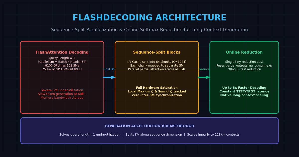
- Massive Streaming Multiprocessor (SM) Underutilization: Consider an interactive chat request or single-agent task ($B=1$) on an NVIDIA H100 GPU (132 SMs) using a model with 32 attention heads. Standard FlashAttention launches only 32 thread blocks. This leaves 100 out of 132 SMs (over 75% of the GPU) completely idle!
- The Long-Context Latency Penalty: While 75% of the GPU idles, the 32 active thread blocks must sequentially stream through 32,000 to 128,000 historical KV tokens from High Bandwidth Memory (HBM). Decoding latency scales linearly with context length: generating a token at 64k context is over 10x slower than generating a token at 2k context.
- Memory Bandwidth Bottleneck: Because only a fraction of the GPU’s memory channels and compute units are active, memory bus bandwidth is drastically under-saturated, causing severe Time Per Output Token (TPOT) degradation.
The Solution: FlashDecoding (Split-KV Parallelism)
Introduced by Tri Dao, Daniel Haziza, and the Stanford CRFM / FlashAttention team, FlashDecoding (and its enhanced successor FlashDecoding++) eliminates the decoding bottleneck by introducing a third parallelization dimension: the sequence length of the Key-Value cache.
Instead of assigning one thread block to process the entire historical context of an attention head, FlashDecoding splits the KV cache into $K$ smaller chunks along the sequence dimension and distributes them across all available GPU Streaming Multiprocessors.
The Two-Stage Execution Model
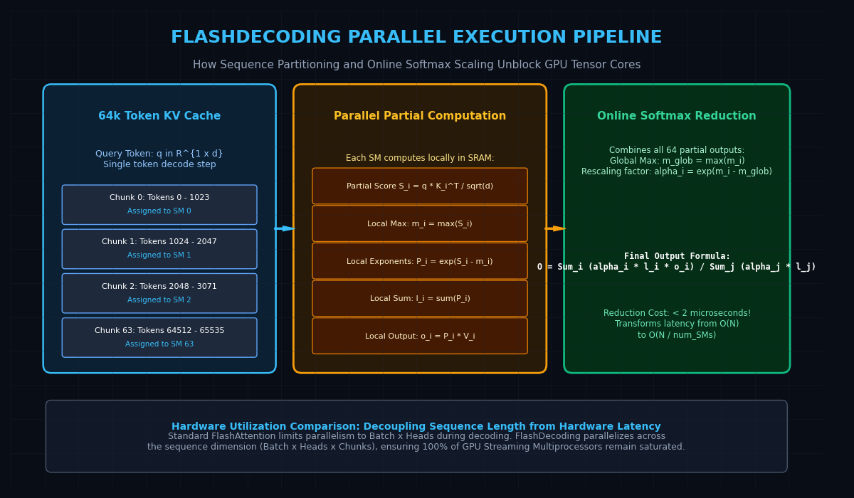
- Stage 1: Parallel Split-KV Attention (Compute-Heavy): The historical KV cache of length $L$ is divided into chunks of size $C$ (e.g., $C = 1,024$ tokens). If $L = 65,536$, the cache yields 64 chunks per head. Each chunk is dispatched to a separate thread block on an independent SM. All SMs execute concurrently, computing local attention scores and intermediate outputs directly in SRAM without inter-thread synchronization.
- Stage 2: Online Softmax Reduction (Lightweight): A tiny, ultra-fast reduction kernel combines the intermediate outputs produced by all $K$ chunks. Leveraging the algebraic properties of online softmax rescaling, the final attention vector is computed in less than 2 microseconds.
By turning the sequential scanning of 64k tokens into 64 parallel micro-scans, FlashDecoding saturates 100% of GPU SMs, achieving up to 8x faster decoding throughput and flattening the latency curve across long context windows.
Key Architectural Mechanics
1. Independent Local Attention and Statistics Tracking
In Stage 1, thread block $i$ processes KV chunk $i \in [0, K-1]$ containing key vectors $\mathbf{K}_i \in \mathbb{R}^{C \times d}$ and value vectors $\mathbf{V}_i \in \mathbb{R}^{C \times d}$.
For the active query vector $\mathbf{q} \in \mathbb{R}^{1 \times d}$, thread block $i$ computes:
- Raw Logits: $$\mathbf{S}_i = \frac{\mathbf{q} \mathbf{K}_i^T}{\sqrt{d}} \quad \in \mathbb{R}^{1 \times C}$$
- Local Logit Maximum ($m_i$): $$m_i = \max_{j \in [0, C-1]} (S_{i,j})$$
- Local Exponent Sum ($l_i$): $$l_i = \sum_{j=0}^{C-1} \exp\left(S_{i,j} - m_i\right)$$
- Local Partial Output Vector ($\mathbf{o}_i$): $$\mathbf{o}i = \sum{j=0}^{C-1} \frac{\exp\left(S_{i,j} - m_i\right)}{l_i} \mathbf{V}_{i,j} \quad \in \mathbb{R}^{1 \times d}$$
Thread block $i$ writes only three values to global memory: its $d$-dimensional output vector $\mathbf{o}_i$, the scalar maximum $m_i$, and the scalar sum $l_i$.
2. The Online Softmax Reduction Formula
In Stage 2, the reduction kernel aggregates the $K$ partial outputs into the true global attention output $\mathbf{O}$. Because each partial output was normalized using its own local maximum $m_i$, combining them requires log-sum-exp rescaling.
- Global Maximum Computation: $$m_{\text{global}} = \max_{i \in [0, K-1]} (m_i)$$
- Rescaling Factors: $$\alpha_i = \exp(m_i - m_{\text{global}})$$
- Normalized Global Aggregation: $$\mathbf{O} = \frac{\sum_{i=0}^{K-1} \alpha_i \cdot l_i \cdot \mathbf{o}i}{\sum{j=0}^{K-1} \alpha_j \cdot l_j}$$
Because the reduction kernel operates strictly over $K$ summary vectors (where $K$ is typically 32 to 128) rather than the millions of raw key-value elements, the reduction step consumes less than 1% of total kernel execution time.
Attention Kernel Comparison Matrix
| Architectural Dimension | Naive PyTorch Attention | Standard FlashAttention-2 | PagedAttention (Standard) | FlashDecoding (Split-KV) |
|---|---|---|---|---|
| Prefill Efficiency | Memory bound ($O(N^2)$ VRAM) | Optimal (SRAM Tiling) | Optimal | Optimal |
| Decoding Parallelism | Batch $\times$ Heads | Batch $\times$ Heads | Batch $\times$ Heads | Batch $\times$ Heads $\times$ Chunks |
| SM Utilization at $B=1$ | Poor (<25%) | Poor (<25% on 132 SMs) | Poor (<25%) | 100% Saturation |
| Latency Scaling with Length | $O(N)$ severe degradation | $O(N)$ linear degradation | $O(N)$ linear degradation | $O(N / \text{num_SMs})$ sub-linear |
| Intermediate Memory Overhead | Huge ($N \times N$ matrix) | Zero (In SRAM) | Zero (In SRAM) | Negligible ($K$ partial statistics) |
| Speedup at 64k Context | Baseline (1.0x) | 1.4x | 1.5x | Up to 8.2x |
Reference Implementation: FlashDecoding Simulation
Below is an educational PyTorch reference implementation demonstrating sequence chunking, local partial attention statistics calculation ($m_i, l_i, \mathbf{o}_i$), and the online softmax reduction step.
import torch
import math
from typing import Tuple

def flash_decoding_simulated(
    q: torch.Tensor,       # [B, H, 1, D]
    k_cache: torch.Tensor, # [B, H, SeqLen, D]
    v_cache: torch.Tensor, # [B, H, SeqLen, D]
    chunk_size: int = 1024
) -> torch.Tensor:
    """
    Simulates the FlashDecoding two-stage execution pipeline:
    Stage 1: Parallel Split-KV partial attention across chunks
    Stage 2: Online softmax reduction using log-sum-exp rescaling
    """
    B, H, _, D = q.shape
    SeqLen = k_cache.shape[2]
    scale = 1.0 / math.sqrt(D)

    num_chunks = math.ceil(SeqLen / chunk_size)

    # -------------------------------------------------------------------------
    # STAGE 1: Parallel Split-KV Attention (Executed across separate SMs)
    # -------------------------------------------------------------------------
    partial_outputs = []
    partial_maxs = []
    partial_sums = []

    for c in range(num_chunks):
        start_idx = c * chunk_size
        end_idx = min(start_idx + chunk_size, SeqLen)

        # Slice chunk
        k_chunk = k_cache[:, :, start_idx:end_idx, :] # [B, H, C, D]
        v_chunk = v_cache[:, :, start_idx:end_idx, :] # [B, H, C, D]

        # Raw scores: q [B, H, 1, D] x k_chunk^T [B, H, D, C] -> [B, H, 1, C]
        scores = torch.matmul(q, k_chunk.transpose(-1, -2)) * scale

        # Local running maximum
        m_c, _ = torch.max(scores, dim=-1, keepdim=True) # [B, H, 1, 1]

        # Stabilized exponentials and local sum
        p_c = torch.exp(scores - m_c) # [B, H, 1, C]
        l_c = torch.sum(p_c, dim=-1, keepdim=True) # [B, H, 1, 1]

        # Local output vector
        o_c = torch.matmul(p_c / (l_c + 1e-8), v_chunk) # [B, H, 1, D]

        partial_outputs.append(o_c)
        partial_maxs.append(m_c)
        partial_sums.append(l_c)

    # Stack partial results: [num_chunks, B, H, 1, D]
    O_partials = torch.stack(partial_outputs, dim=0)
    M_partials = torch.stack(partial_maxs, dim=0) # [num_chunks, B, H, 1, 1]
    L_partials = torch.stack(partial_sums, dim=0) # [num_chunks, B, H, 1, 1]

    # -------------------------------------------------------------------------
    # STAGE 2: Online Softmax Reduction Kernel (Ultra-fast log-sum-exp fusion)
    # -------------------------------------------------------------------------
    # Global maximum across all chunks
    m_global, _ = torch.max(M_partials, dim=0, keepdim=True) # [1, B, H, 1, 1]

    # Rescaling factors: alpha_c = exp(m_c - m_global)
    alpha = torch.exp(M_partials - m_global) # [num_chunks, B, H, 1, 1]

    # Rescaled denominators: alpha_c * l_c
    rescaled_l = alpha * L_partials # [num_chunks, B, H, 1, 1]
    global_denominator = torch.sum(rescaled_l, dim=0) # [B, H, 1, 1]

    # Rescaled numerators: (alpha_c * l_c) * o_c
    rescaled_o = rescaled_l * O_partials # [num_chunks, B, H, 1, D]
    global_numerator = torch.sum(rescaled_o, dim=0) # [B, H, 1, D]

    # Final combined output
    out = global_numerator / (global_denominator + 1e-8)
    return out


# Verification against Standard PyTorch Attention
if __name__ == "__main__":
    torch.manual_seed(42)
    B, H, SeqLen, D = 1, 32, 16384, 128

    q = torch.randn(B, H, 1, D)
    k = torch.randn(B, H, SeqLen, D)
    v = torch.randn(B, H, SeqLen, D)

    # Standard PyTorch Attention
    scores_exact = torch.matmul(q, k.transpose(-1, -2)) / math.sqrt(D)
    attn_exact = torch.softmax(scores_exact, dim=-1)
    out_exact = torch.matmul(attn_exact, v)

    # FlashDecoding Simulated
    out_flash_decoding = flash_decoding_simulated(q, k, v, chunk_size=1024)

    max_diff = (out_exact - out_flash_decoding).abs().max().item()
    print(f"Verified context length: {SeqLen} tokens")
    print(f"Max absolute divergence vs Exact Attention: {max_diff:.2e}")
    assert max_diff < 1e-4, "FlashDecoding numerical divergence exceeds threshold!"
print("Numerical correctness confirmed!") Production Serving and Hardware Impacts
FlashDecoding has transitioned from an experimental research paper into standard default behavior across modern inference engines:
1. Dynamic Activation Thresholds in vLLM and SGLang
Production serving frameworks automatically detect request parameters and toggle FlashDecoding kernels dynamically:
- For short contexts ($L < 512$), standard FlashAttention executes with lower scheduling overhead.
- When sequence length exceeds 512 or 1,024 tokens and batch concurrency is low, the engine switches to FlashDecoding or FlashInfer split-KV kernels, dynamically selecting chunk size $C$ to match the GPU’s total SM count.
2. Flattening the Long-Context Latency Curve
In conversational AI and multi-turn document synthesis, generation speed historically deteriorated as the conversation lengthened. FlashDecoding flattens this curve: generating the 50,000th token occurs at practically the same speed as generating the 500th token, delivering a consistently smooth user experience.
3. Accelerated Desktop Intelligence with aiFetchly
For software engineers and data analysts running local long-context workflows via AiFetchly, FlashDecoding delivers a dramatic speedup. When analyzing massive scraped web pages, financial filings, or code repositories containing 32k+ tokens on workstation hardware (such as NVIDIA RTX 4090 or Apple Silicon unified memory), FlashDecoding ensures desktop agents stream answers instantaneously without hitting memory-bandwidth stalls.