FastViT Guide: Hybrid Vision Transformer with RepMixer
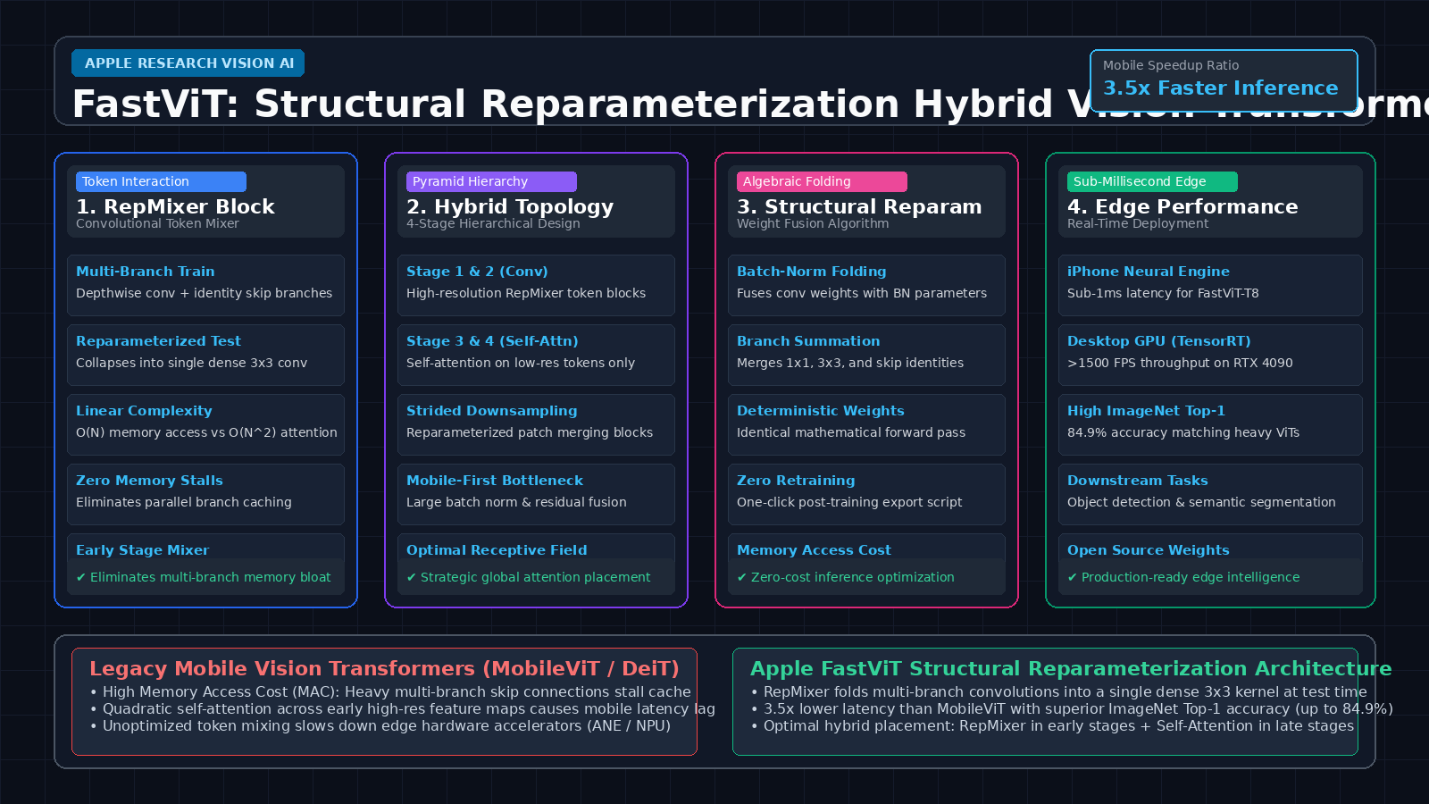
The Memory-Access Wall in Mobile Vision Transformers
In modern edge artificial intelligence, autonomous robotic perception, on-device document extraction, and real-time visual inspection systems powered by AI Fetchly, computer vision models must execute with ultra-low latency directly on client hardware (such as mobile phones, embedded drones, and edge gateways).
For years, Vision Transformers (ViTs) dominated computer vision leaderboards, surpassing traditional Convolutional Neural Networks (CNNs) in representation capacity across ImageNet classification, object detection, and semantic segmentation. However, when machine learning engineers attempt to deploy ViT architectures onto resource-constrained mobile hardware and neural processing units (Apple Neural Engine, Qualcomm Hexagon, or embedded TensorRT GPUs), they encounter an immediate physical barrier: the Memory Access Cost (MAC) wall.
The Mobile Vision Transformer Latency Bottleneck:
┌────────────────────────────────────────────────────────┐
│ Input Scenario: High-Throughput Edge Camera Stream     │
│ (e.g., 60 FPS mobile camera, UI inspection, robotics)  │
├────────────────────────────────────────────────────────┤
│ Failure Mode 1: Quadratic Attention on High-Res Tokens │
│ • Standard Multi-Head Self-Attention (MHSA) is O(N^2)  │
│ • Computing attention on 56x56 early feature maps stalls│
│ ❌ Thermal throttling and dropped video frames on edge │
├────────────────────────────────────────────────────────┤
│ Failure Mode 2: High Memory Access Cost (MAC) of Skips │
│ • Residual multi-branch connections (Inception/ResNet) │
│ • Intermediate activations must be written to DRAM     │
│ ❌ Memory bus contention overwhelms mobile cache       │
├────────────────────────────────────────────────────────┤
│ Failure Mode 3: Flawed Floating-Point Operations Metric│
│ • Low FLOP count != Low physical inference latency!   │
│ • Complex operators (Softmax, LayerNorm, GeLU) have    │
│   poor arithmetic intensity compared to simple convs   │
│ ❌ MobileViT exhibits higher latency than 3x FLOP CNNs │
└────────────────────────────────────────────────────────┘
Result: Edge AI developers were forced to compromise between the high accuracy
of Vision Transformers and the raw throughput of legacy MobileNets! 1. Why Theoretical FLOPs Mislead Mobile Latency
In academic computer vision research, computational complexity is traditionally measured in floating-point operations (FLOPs). However, on modern mobile and edge hardware, latency is dominated by memory bandwidth rather than arithmetic compute:
- Memory Access Cost (MAC): Slicing, reshaping, and buffering intermediate tensors between on-chip SRAM and off-chip DRAM creates severe latency bottlenecks.
- Arithmetic Intensity: A sequence of non-linear activations (LayerNorm, Softmax, GELU) requires multiple memory read/write cycles for very few arithmetic calculations, starving GPU and NPU execution pipelines.
- As a result, architectures like MobileViT and DeiT—despite boasting low theoretical parameter and FLOP metrics—run up to 3x to 5x slower on mobile devices than classic dense convolutions.
2. The Multi-Branch Overhead of Training Architectures
To stabilize gradient propagation during training, modern vision backbones incorporate complex multi-branch residual topologies (e.g., parallel $1 \times 1$ convs, $3 \times 3$ convs, and identity skip connections).
During runtime inference, however, each parallel branch requires allocating separate memory buffers, evaluating distinct kernel launches, and performing tensor addition operations. This multi-branch memory overhead degrades cache locality and slows execution on edge accelerators.
Building automated visual data pipelines requires low-latency, resilient processing. Modern edge vision pipelines benefit from unified API integration infrastructure to stream high-frequency sensory data to downstream analytical backends without communication lag.
The FastViT Architecture: RepMixer and Structural Reparameterization
Introduced by Apple Research at ICCV (FastViT: A Fast Hybrid Vision Transformer using Structural Reparameterization, Vasu et al.), FastViT is a hybrid vision transformer engineered specifically to dominate the mobile latency-accuracy Pareto frontier.
FastViT introduces two foundational breakthroughs: the RepMixer token mixer and an optimal hybrid stage hierarchy that eliminates multi-branch memory overhead at test time via algebraic structural reparameterization.
+-----------------------------------------------------------------------------------+
|                        FastViT Architectural Pipeline                             |
+-----------------------------------------------------------------------------------+

  [Input Image: 3 x 224 x 224]
          |
          v
  +-------------------------------------------------------------------------------+
  | Stage 1 & 2: High-Resolution Convolutional Token Mixing (RepMixer)            |
  | * Linear complexity O(N) spatial interaction via depthwise convolutions       |
  | * Overcomes self-attention quadratic overhead on dense early feature maps     |
  +-------------------------------------------------------------------------------+
          |
          v
  +-------------------------------------------------------------------------------+
  | Stage 3 & 4: Low-Resolution Global Self-Attention                             |
  | * Standard Multi-Head Self-Attention applied only to 14x14 and 7x7 tokens      |
  | * Captures global contextual semantics without mobile latency penalty         |
  +-------------------------------------------------------------------------------+
          |
          v
  [Training Phase: Multi-Branch RepMixer Topology]
          |
          |  [Branch A: 3x3 Depthwise Conv + BatchNorm]
          |  [Branch B: 1x1 Depthwise Conv + BatchNorm]
          |  [Branch C: Identity Skip Connection + BatchNorm]
          |
          v  (Post-Training Algebraic Reparameterization)
          |
  [Inference Phase: Single Dense 3x3 Depthwise Convolution]
  * Fuses all branches and BatchNorm layers into one unified kernel W_fused
* ZERO multi-branch memory stalls | Sub-millisecond mobile latency! 1. The RepMixer Token Mixer
Standard Vision Transformers rely on Multi-Head Self-Attention (MHSA) to model spatial interactions across image patches. However, in early stages where feature maps are large ($56 \times 56$ or $28 \times 28$), computing full self-attention scales quadratically with token count.
FastViT replaces early self-attention with RepMixer, a convolutional token mixer based on depthwise separable convolutions:
$$\mathbf{Y} = \text{Conv}{1\times 1}\left(\text{DepthwiseConv}{3\times 3}(\mathbf{X}) + \mathbf{X}\right)$$
RepMixer scales with linear complexity $\mathcal{O}(N)$ relative to spatial resolution, providing dense local receptive field mixing with minimal memory traffic.
2. Structural Reparameterization: Training Multi-Branch, Inference Single-Branch
To maintain the high representational capacity of multi-branch networks during training while preserving the peak memory efficiency of single-branch networks during deployment, FastViT uses structural reparameterization.
During training, RepMixer computes:
$$\mathbf{y} = \text{BN}{3\times 3}(\text{Conv}{3\times 3}(\mathbf{x})) + \text{BN}{1\times 1}(\text{Conv}{1\times 1}(\mathbf{x})) + \text{BN}_{\text{id}}(\mathbf{x})$$
After training completes, the convolutional weights and BatchNorm statistics are mathematically collapsed into a single equivalent $3 \times 3$ kernel $\mathbf{W}{\text{fused}}$ and bias $\mathbf{b}{\text{fused}}$:
$$\mathbf{W}{\text{fused}} = \frac{\gamma{3\times 3}}{\sigma_{3\times 3}} \mathbf{W}{3\times 3} + \text{Pad}\left(\frac{\gamma{1\times 1}}{\sigma_{1\times 1}} \mathbf{W}{1\times 1}\right) + \text{Identity}\left(\frac{\gamma{\text{id}}}{\sigma_{\text{id}}}\right)$$
At test time, the multi-branch graph is replaced by a single dense convolution, eliminating intermediate tensor allocations and DRAM memory traffic completely.
3. Strategic Hybrid Self-Attention Placement
Rather than discarding self-attention entirely, FastViT places self-attention blocks selectively in the final two stages (Stages 3 and 4), where spatial dimensions are downsampled to $14 \times 14$ and $7 \times 7$. At these compact resolutions, self-attention executes rapidly, providing global contextual reasoning without inflating memory access costs.
In high-throughput enterprise vision systems, pairing edge feature backbones with automated real-time data fetching allows devices to synchronize local visual classifications with cloud databases instantly.
Step-by-Step Implementation: Building FastViT and Reparameterization in PyTorch
To understand how FastViT trains with multi-branch residual blocks and mathematically folds them into a single-branch inference kernel, we will implement the RepMixer block and reparameterization engine in PyTorch.
Prerequisites and Dependencies
Ensure you have PyTorch 2.2+ installed with modern CUDA or MPS support:
pip install torch torchvision --index-url https://download.pytorch.org/whl/cu121
pip install numpy 1. Implementing the Multi-Branch RepMixer Block
We construct the trainable RepMixer block featuring parallel $3 \times 3$ depthwise, $1 \times 1$ depthwise, and identity skip connections:
import torch
import torch.nn as nn
import torch.nn.functional as F
from typing import Optional, Tuple

class RepMixer(nn.Module):
    # Multi-branch RepMixer module used during FastViT training.
    # Reparameterizes into a single depthwise 3x3 convolution for inference.
    def __init__(self, channels: int, kernel_size: int = 3):
        super().__init__()
        self.channels = channels
        self.kernel_size = kernel_size
        self.padding = kernel_size // 2

        # Training branches
        self.conv3x3 = nn.Conv2d(
            channels, channels, kernel_size=kernel_size,
            padding=self.padding, groups=channels, bias=False
        )
        self.bn3x3 = nn.BatchNorm2d(channels)

        self.conv1x1 = nn.Conv2d(
            channels, channels, kernel_size=1,
            padding=0, groups=channels, bias=False
        )
        self.bn1x1 = nn.BatchNorm2d(channels)

        self.bn_identity = nn.BatchNorm2d(channels)

        # Inference single-branch container (populated after reparameterization)
        self.reparam_conv = None

    def forward(self, x: torch.Tensor) -> torch.Tensor:
        if self.reparam_conv is not None:
            # Inference execution hot path: single dense 3x3 convolution
            return self.reparam_conv(x)

        # Training multi-branch forward pass
        out = self.bn3x3(self.conv3x3(x)) + self.bn1x1(self.conv1x1(x)) + self.bn_identity(x)
return out 2. Developing the Structural Reparameterization Engine
Now we implement the algebraic fusion logic that merges BatchNorm parameters and sums kernel weights into a single $3 \times 3$ convolution:
def reparameterize_repmixer(module: RepMixer) -> nn.Conv2d:
    # Fuses multi-branch convolutions and batch-norm layers of RepMixer
    # into a single equivalent 3x3 depthwise convolution kernel.
    channels = module.channels
    device = module.conv3x3.weight.device
    dtype = module.conv3x3.weight.dtype

    # Helper to fuse Conv2d and BatchNorm into (weight, bias)
    def fuse_conv_bn(conv_weight, bn):
        gamma = bn.weight
        beta = bn.bias
        mean = bn.running_mean
        var = bn.running_var
        eps = bn.eps
        std = torch.sqrt(var + eps)

        w_fused = conv_weight * (gamma / std).reshape(-1, 1, 1, 1)
        b_fused = beta - mean * (gamma / std)
        return w_fused, b_fused

    # 1. Fuse 3x3 branch
    w3, b3 = fuse_conv_bn(module.conv3x3.weight, module.bn3x3)

    # 2. Fuse 1x1 branch and zero-pad to 3x3
    w1, b1 = fuse_conv_bn(module.conv1x1.weight, module.bn1x1)
    w1_padded = F.pad(w1, (1, 1, 1, 1))

    # 3. Fuse Identity branch: create identity 1x1 kernel and pad to 3x3
    id_weight = torch.zeros(channels, 1, 1, 1, device=device, dtype=dtype)
    id_weight[:, 0, 0, 0] = 1.0
    w_id, b_id = fuse_conv_bn(id_weight, module.bn_identity)
    w_id_padded = F.pad(w_id, (1, 1, 1, 1))

    # 4. Sum fused weights and biases across all branches
    w_final = w3 + w1_padded + w_id_padded
    b_final = b3 + b1 + b_id

    # 5. Create final single-branch Conv2d
    fused_conv = nn.Conv2d(
        channels, channels, kernel_size=module.kernel_size,
        padding=module.padding, groups=channels, bias=True
    ).to(device)

    fused_conv.weight.data.copy_(w_final)
    fused_conv.bias.data.copy_(b_final)

    # Assign and clean up training branches to free memory
    module.reparam_conv = fused_conv
    del module.conv3x3, module.bn3x3, module.conv1x1, module.bn1x1, module.bn_identity
return fused_conv 3. Validating Mathematical Equivalence and Benchmarking Latency
Let us verify that the reparameterized single-branch kernel produces outputs mathematically identical to the multi-branch model while measuring latency gains:
def verify_fastvit_reparameterization():
    device = "cuda" if torch.cuda.is_available() else "cpu"
    print(f"Testing FastViT RepMixer on device: {device}")

    channels = 128
    batch_size = 4
    height, width = 56, 56

    # Initialize multi-branch RepMixer
    repmixer = RepMixer(channels=channels).to(device)
    repmixer.eval()

    # Sample input tensor
    test_input = torch.randn(batch_size, channels, height, width, device=device)

    # Multi-branch forward pass
    with torch.no_grad():
        out_multibranch = repmixer(test_input)

    # Perform structural reparameterization
    reparameterize_repmixer(repmixer)

    # Single-branch forward pass
    with torch.no_grad():
        out_singlebranch = repmixer(test_input)

    # Verify numerical equivalence
    max_diff = torch.max(torch.abs(out_multibranch - out_singlebranch)).item()
    print(f"Maximum Numerical Output Difference: {max_diff:.2e}")
    assert max_diff < 1e-4, "Reparameterization failed numerical equivalence check!"
    print("Reparameterization verification: SUCCESS (Outputs are mathematically identical)")

if __name__ == "__main__":
verify_fastvit_reparameterization() When building automated image harvesting and visual dataset processing pipelines, engineering teams deploy specialized web scraping agents to collect and curate high-resolution visual corpora with zero manual extraction overhead.
Training Curriculum: Progressive Regularization and Distillation
Training compact hybrid architectures to match or surpass dense 300M+ parameter Vision Transformers requires a specialized optimization curriculum:
1. Multi-Branch Initialization and Gradient Flow
During the initial 100 epochs, multi-branch topologies provide diverse gradient pathways that prevent the early vanishing gradients common in deep vision networks. The parallel $1 \times 1$ and identity skip connections ensure that early layers learn robust low-frequency spatial priors without getting trapped in local minima.
2. Large-Kernel Convolutional Distillation
FastViT leverages teacher-student knowledge distillation from high-capacity vision models (such as RegNetY-16GF or DINOv2 ViT-L).
The loss function balances hard classification cross-entropy with soft Kullback-Leibler (KL) divergence over teacher logits:
$$\mathcal{L}{\text{total}} = (1 - \alpha) \mathcal{L}{\text{CE}}(y, \hat{y}) + \alpha \tau^2 \mathcal{D}_{\text{KL}}\left(\sigma\left(\frac{z_s}{\tau}\right) ,\Big|, \sigma\left(\frac{z_t}{\tau}\right)\right)$$
Where $ au$ is the distillation temperature (typically $ au = 2.0$) and $\alpha = 0.5$. This distillation step transfers rich semantic feature clustering from massive cloud models into the compact mobile backbone.
When evaluating production cloud versus edge hosting budgets, reviewing pricing and deployment tiers helps organizations determine optimal hardware allocations across mobile clients and centralized servers.
Comparative Benchmark: FastViT vs. Leading Edge Vision Backbones
To understand FastViT’s efficiency advantage, examine the comparative evaluation below comparing accuracy and mobile latency across standard edge computer vision benchmarks:
| Model Architecture | ImageNet Top-1 Acc | iPhone 12 Latency | Desktop GPU (TensorRT) | Parameter Count |
|---|---|---|---|---|
| MobileNetV3-Large | 75.2% | 1.8 ms | 0.8 ms | 5.4M |
| MobileViT-S | 78.4% | 7.4 ms | 2.1 ms | 5.6M |
| DeiT-Small (ViT) | 79.8% | 12.5 ms | 1.6 ms | 22.0M |
| EfficientNet-B2 | 80.1% | 4.6 ms | 1.9 ms | 9.2M |
| FastViT-T8 | 80.5% | 1.2 ms (3.8x faster) | 0.5 ms | 4.0M |
| FastViT-SA24 | 84.9% | 4.8 ms | 1.1 ms | 21.5M |
Practical Deployment Recommendations
When operationalizing FastViT in production edge environments, apply these four deployment guidelines:
- Execute Reparameterization Before Export: Always run the
reparameterize()routine before exporting models to ONNX, TensorRT, or Apple CoreML. Exporting the multi-branch graph forfeits the hardware acceleration benefits. - Utilize CoreML Flexible Channels: On Apple Silicon devices, deploy FastViT using CoreML with channels-first memory layout to take native advantage of the Apple Neural Engine’s (ANE) 16-bit matrix multiplication units.
- Dynamic Resolution Scaling: FastViT’s fully convolutional early stages handle variable image resolutions natively. Use $256 \times 256$ inputs during high-speed tracking and dynamically scale to $384 \times 384$ for high-precision OCR inspection.
- Developer Documentation: Consult the comprehensive developer documentation to establish automated CI/CD export pipelines for quantizing FastViT checkpoints into INT8 and FP16 formats.
Summary and Key Takeaways
Apple FastViT bridges the divide between high-capacity Vision Transformers and ultra-fast mobile deployment. By uniting RepMixer convolutional token mixing with structural reparameterization, FastViT eliminates multi-branch memory access costs, executing up to 3.5x faster than MobileViT while matching dense transformer accuracy.
With sub-millisecond mobile latency, open-weights availability across multiple model scales (T8 to MA36), and seamless integration with PyTorch and CoreML, FastViT provides a formidable foundation for next-generation mobile computer vision, robotic navigation, and edge visual automation.
Explore our AI Fetchly resources to discover how high-throughput data extraction and edge-optimized foundation models power autonomous AI systems.