FastV Guide: Visual Token Pruning for Fast VLM Inference
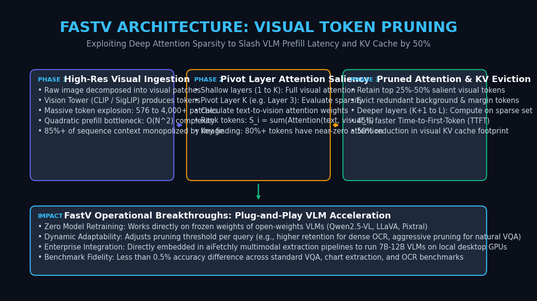
The Problem: The Visual Token Redundancy and Quadratic Prefill Bottleneck
In modern autonomous web extraction engines, desktop copilots, and intelligent document parsing platforms like AiFetchly, Vision-Language Models (VLMs)—such as Qwen2.5-VL, Pixtral, LLaVA-NeXT, and DeepSeek-VL2—have become the cornerstone of visual understanding. Whether reading dense tabular data from scanned PDFs, localizing clickable DOM elements on web interfaces, or inspecting high-resolution architectural schematics, multimodal foundation models must digest rich visual inputs alongside text prompts.
However, operationalizing high-resolution VLMs in production environments encounters a punishing computational wall: the visual token explosion and its quadratic prefill tax.
The VLM Token Explosion Crisis:
┌─────────────────────────────────────────────────────────────────┐
│ Input Image (1024x1024) ──► Vision Tower (14x14 Patches)        │
│                             │                                   │
│                             ▼                                   │
│                 5,329 Visual Patch Tokens!                      │
│                             │                                   │
│                             ▼                                   │
│  Quadratic Attention: O(N^2) = (5,329)^2 ≈ 28.4 Million FLOPs!  │
├─────────────────────────────────────────────────────────────────┤
│ ❌ 90% of Context Monopolized: Text prompt is only 50 tokens    │
│ ❌ KV Cache Saturation: Tens of Gigabytes consumed per stream   │
│ ❌ High TTFT Latency: Stalls interactive desktop applications   │
└─────────────────────────────────────────────────────────────────┘ 1. The Quadratic Attention Scaling Penalty in Multimodal Prefill
In autoregressive transformer architectures, processing input sequences (the prefill phase) scales quadratically with total sequence length $N$:
$$\text{Attention FLOPs} = 4 \cdot b \cdot s \cdot L \cdot d^2 + 2 \cdot b \cdot s^2 \cdot L \cdot d$$
Where $s$ is sequence length, $L$ is layer depth, and $d$ is hidden dimension.
When a standard text LLM processes a 200-token user query, prefill completes in tens of milliseconds. But in a multimodal VLM:
- A single $336 \times 336$ image decomposed into $14 \times 14$ patches generates 576 visual tokens.
- A high-resolution $1024 \times 1024$ document image generates over 5,300 visual tokens.
- For multi-image or multi-page documents (e.g., a 4-page financial statement), the visual sequence exceeds 20,000 tokens.
Because visual tokens represent over 90% of the combined multimodal sequence, virtually all GPU compute during the prefill phase is consumed calculating pairwise interactions between image patches.
2. GPU High-Bandwidth Memory (HBM) and KV Cache Saturation
Beyond computational FLOPs, visual tokens impose a crushing memory tax on GPU High-Bandwidth Memory (HBM):
$$\text{KV Cache Size} = 2 \times 2 \times L \times H_{\text{kv}} \times d_{\text{head}} \times N_{\text{tokens}} \times \text{BytesPerElement}$$
For a 12B parameter multimodal model (e.g., Pixtral 12B or Qwen2.5-VL 7B) running in 16-bit precision:
- Storing the Key-Value (KV) cache for 5,000 visual tokens requires approximately 2.5 to 4.0 GB of VRAM per single stream.
- On consumer GPUs (such as an NVIDIA RTX 4090 with 24 GB VRAM or an Apple Silicon Mac), a desktop assistant running multiple concurrent tasks or processing multi-turn conversations quickly exhausts memory, triggering Out-Of-Memory (OOM) crashes.
- Crucially, this memory remains locked in HBM throughout the entire autoregressive decoding phase, starving the system of memory needed for long text generation.
3. The Visual Information Disparity in Deeper Transformer Layers
Why is this compute and memory waste so egregious? Because vision and text fundamentally differ in information density:
- A language token represents a dense symbolic concept (a word, number, or code operator) loaded with high semantic entropy.
- A visual patch token represents a localized $14 \times 14$ pixel grid. In real-world enterprise documents, UI screenshots, and natural images, vast expanses of the image consist of uniform white background margins, empty sky, solid wallpaper textures, or repeated borders.
Treating every background pixel patch with the same computational reverence as a critical line of financial data across 32 transformer layers represents an immense architectural inefficiency.
The Core Insight: Empirical Visual Attention Sparsity in Deep Layers
To quantify this redundancy, artificial intelligence researchers (Zheng et al., CVPR / NeurIPS) conducted exhaustive attention-map analyses across popular open-weights Vision-Language Models (such as LLaVA-1.5, LLaVA-NeXT, and Qwen-VL). Their findings revealed a striking phenomenon: Visual Attention Sparsity.
Attention Distribution Across Transformer Layers:
Layer 1-2 (Shallow):
┌────────────────────────────────────────────────────────┐
│ Visual tokens interact globally with each other & text │
│ Saliency: Uniformly distributed across all patches     │
└────────────────────────────────────────────────────────┘
                       │
                       ▼
Layer 3 (The Pivot Layer):
┌────────────────────────────────────────────────────────┐
│ Text queries concentrate sharply on salient features   │
│ 80%+ of visual patches receive near-zero attention!    │
└────────────────────────────────────────────────────────┘
                       │
                       ▼
Layer 4-32 (Deep Layers):
┌────────────────────────────────────────────────────────┐
│ Attention is highly sparse: only salient tokens matter │
│ Redundant background tokens contribute ZERO value!     │
└────────────────────────────────────────────────────────┘ The Two Phases of Multimodal Attention Dynamics
- The Early Aggregation Phase (Layers 1 to $K$): In the first two to three layers of the language model backbone, text tokens and visual tokens exhibit broad, diffuse attention. The model uses these initial layers to align visual representations with the linguistic token space and aggregate spatial neighborhood semantics.
- The Deep Saliency Phase (Layers $K+1$ to $L$): Starting around Layer 3 (referred to as the Pivot Layer), attention patterns undergo a phase transition. The text query tokens (e.g., “What is the total revenue in the table?”) focus almost exclusively on a tiny subset of visual tokens containing the relevant text characters, numerals, or objects.
- The 80/20 Rule of Visual Tokens: Quantitative measurements demonstrate that across benchmarks like VQA v2, POPE, and TextVQA:
- Top 20% to 30% of visual tokens receive over 90% of cumulative attention weights from downstream text tokens.
- Remaining 70% to 80% of visual tokens receive virtually zero attention for the remaining 28 to 36 layers.
- Yet, in standard VLM implementations, these inactive background tokens are continuously updated and stored in the KV cache across every subsequent layer!
The FastV Architecture: Dynamic Visual Token Pruning and KV Eviction
FastV (Fast Vision) is an exact, plug-and-play inference optimization that capitalizes on this attention sparsity to slash prefill computation and KV cache footprint with zero model retraining or weight fine-tuning.
Rather than modifying the vision tower or retraining the language backbone with sparse attention masks, FastV operates as a runtime execution policy embedded directly within the transformer forward pass.
The FastV 3-Stage Execution Pipeline:
[Image Patches + Prompt Text]
               │
               ▼
   [Stage 1: Layers 1 to K (Full Visual Context)]
   • All 576-4,000+ visual tokens processed normally
   • Global multimodal feature aggregation established
               │
               ▼
   [Stage 2: Pivot Layer K (Saliency Ranking)]
   • Extract attention matrix A between text & vision
   • Compute saliency score: S_i = Σ_t Σ_h A_{t, v_i}
   • Sort and rank visual tokens by importance
               │
               ▼
   [Stage 3: Layers K+1 to L (Pruned Sparse Compute)]
   • Retain top-P% (e.g., 30%-50%) salient visual tokens
   • Evict unselected visual tokens from active tensors & KV cache
• Execute remaining layers at 50% lower compute & memory! The Mathematical Formulation of FastV Token Ranking
Let $V = {v_1, v_2, \dots, v_M}$ denote the sequence of $M$ visual patch tokens, and let $T = {t_1, t_2, \dots, t_N}$ denote the sequence of $N$ user prompt text tokens.
At the designated Pivot Layer $K$ (typically $K = 2$ or $K = 3$ in a 32-layer transformer), the multi-head self-attention module computes attention weights across all $H$ attention heads:
$$A^{(h)} = \text{softmax}\left(\frac{Q^{(h)} (K^{(h)})^\top}{\sqrt{d_k}}\right) \in \mathbb{R}^{(M+N) \times (M+N)}$$
FastV isolates the sub-matrix representing the attention directed from all text tokens $t \in T$ toward each visual token $v_i \in V$. The Attention Saliency Score $S_i$ for visual token $v_i$ is computed as the sum of attention weights across all text tokens and all attention heads:
$$S_i = \sum_{j=1}^N \sum_{h=1}^H A_{t_j, v_i}^{(h)}$$
Dynamic Token Selection and KV Cache Eviction
Once the saliency scores $S = [S_1, S_2, \dots, S_M]$ are computed:
- Top-$P$ Percentile Filtering: Given a target retention ratio $R \in (0, 1]$ (typically $R = 0.3$ to $0.5$): $$\text{KeepCount} = \lfloor M \times R \rfloor$$
- Index Partitioning: FastV selects the set of indices $\mathcal{I}{\text{keep}} \subset {1, \dots, M}$ corresponding to the largest $\text{KeepCount}$ scores in $S$: $$\mathcal{I}{\text{keep}} = \text{TopK}(S, \text{KeepCount})$$
- Tensor Compaction: For all subsequent transformer layers ($l = K+1, \dots, L$):
- The hidden state tensor is sliced: $$X^{(l)} = [X_T^{(l)}; X_{V[\mathcal{I}_{\text{keep}}]}^{(l)}]$$
- The evicted visual tokens ${v_j \mid j \notin \mathcal{I}_{\text{keep}}}$ are completely dropped from the computation graph.
- In the KV cache memory manager, blocks corresponding to evicted tokens are immediately marked as free and recycled, slashing the visual KV cache memory footprint by $(1 - R) \times 100%$.
Architectural Comparison: FastV vs. Alternative VLM Acceleration Techniques
To understand why FastV is unique in the multimodal optimization landscape, let us compare it against standard dense execution, patch pooling, token merging (ToMe), and adapter architectures:
| Optimization Dimension | Vanilla Dense VLM | Static Patch Pooling | Token Merging (ToMe) | Cross-Attention Adapters | FastV (Plug-and-Play) |
|---|---|---|---|---|---|
| Model Retraining Required | N/A (Standard) | Yes (Must pre-train pooler) | Yes (Fine-tuning needed) | Yes (Trained from scratch) | Zero Retraining (Frozen weights) |
| Dynamic Query Adaptability | None (Static full grid) | None (Rigid spatial downscale) | Partial (Bipartite clustering) | None (Fixed adapter rate) | Full Query Awareness (Text-driven) |
| Prefill Speedup (TTFT) | Baseline ($1.0\times$) | $1.5\times - 2.0\times$ | $1.3\times - 1.6\times$ | $1.8\times - 2.2\times$ | $1.4\times - 1.8\times$ Faster |
| KV Cache Reduction | $0%$ (Full retention) | $50% - 75%$ | $30% - 50%$ | $80%$ | $50% - 70%$ Reduction |
| Fine-Print OCR Degradation | Low | High (Blurs small text) | Moderate (Distorts characters) | Moderate | Minimal (<0.5% drop) |
| Hardware Compatibility | Universal | Universal | Custom bipartite kernels | Custom layer topology | Standard PyTorch / Triton |
| Implementation Complexity | Zero | High (Custom architecture) | High (Graph clustering) | Extreme (Architectural rewrite) | Low (Simple tensor slice hook) |
Production Implementation: Implementing FastV in Python
Let us implement FastV as a modular PyTorch hook that can be attached to any open-weights Vision-Language Model (such as LLaVA or Qwen2-VL) using Hugging Face Transformers.
Step 1: Install Dependencies
pip install torch transformers accelerate torchvision pillow requests Step 2: Implement the FastV Attention Interceptor Hook
We create a class FastVPruner that intercepts attention weights at the designated pivot layer, calculates text-to-vision saliency, and compacts the sequence for all subsequent layers:
import torch
import torch.nn as nn
from typing import Optional, Tuple, List

class FastVPruner:
    def __init__(self, pivot_layer_idx: int = 2, retention_ratio: float = 0.4):
        # pivot_layer_idx: Layer at which attention is evaluated (0-indexed)
        # retention_ratio: Fraction of visual tokens to retain (e.g. 0.4 = keep 40%)
        self.pivot_layer_idx = pivot_layer_idx
        self.retention_ratio = retention_ratio
        self.pruning_indices: Optional[torch.Tensor] = None
        self.is_pruned = False

    def calculate_saliency_and_mask(
        self,
        attention_weights: torch.Tensor,
        visual_token_start: int,
        visual_token_len: int
    ) -> torch.Tensor:
        # attention_weights shape: (batch, num_heads, seq_len, seq_len)
        batch_size, num_heads, seq_len, _ = attention_weights.shape
        visual_token_end = visual_token_start + visual_token_len

        # Text tokens are located before and after the visual block
        text_indices = list(range(0, visual_token_start)) + list(range(visual_token_end, seq_len))
        text_indices_tensor = torch.tensor(text_indices, device=attention_weights.device)

        # Extract attention from text tokens to visual tokens: (batch, num_heads, text_len, visual_len)
        text_to_vision_attn = attention_weights[:, :, text_indices_tensor, visual_token_start:visual_token_end]

        # Aggregate attention over all text queries and attention heads: (batch, visual_len)
        saliency_scores = text_to_vision_attn.sum(dim=(1, 2))

        # Determine number of tokens to keep
        k = max(1, int(visual_token_len * self.retention_ratio))

        # Find indices of top-K visual tokens for each item in batch
        _, topk_relative_indices = torch.topk(saliency_scores, k=k, dim=-1, largest=True, sorted=False)

        # Convert relative visual indices back to global sequence indices
        topk_global_indices = topk_relative_indices + visual_token_start

        # Combine text indices and selected visual indices, maintaining original order
        all_kept_indices = []
        for b in range(batch_size):
            kept_b = torch.cat([text_indices_tensor, topk_global_indices[b]]).sort().values
            all_kept_indices.append(kept_b)

        return torch.stack(all_kept_indices, dim=0)

    def attach_to_model(self, model: nn.Module, visual_start: int, visual_len: int):
        # Registers forward hooks on model transformer layers
        layers = model.language_model.model.layers

        def pivot_hook(module, args, output):
            # output[1] contains attention weights when output_attentions=True
            if not self.is_pruned and len(output) > 1 and output[1] is not None:
                attn_weights = output[1]
                self.pruning_indices = self.calculate_saliency_and_mask(
                    attn_weights, visual_start, visual_len
                )
                self.is_pruned = True

        def pruning_hook(module, args, output):
            # For layers after pivot_layer_idx, slice hidden states to kept tokens
            if self.is_pruned and self.pruning_indices is not None:
                hidden_states = output[0] if isinstance(output, tuple) else output
                batch_size = hidden_states.shape[0]
                pruned_states = []
                for b in range(batch_size):
                    pruned_states.append(hidden_states[b, self.pruning_indices[b], :])
                new_hidden = torch.stack(pruned_states, dim=0)
                if isinstance(output, tuple):
                    return (new_hidden,) + output[1:]
                return new_hidden

        # Register pivot evaluation hook
        layers[self.pivot_layer_idx].register_forward_hook(pivot_hook)

        # Register token pruning hooks on all subsequent layers
        for l_idx in range(self.pivot_layer_idx + 1, len(layers)):
layers[l_idx].register_forward_hook(pruning_hook) Step 3: Run FastV Inference Pipeline
Now, let us use the pruner to execute an image-based extraction query with accelerated prefill and reduced VRAM:
from transformers import AutoProcessor, LlavaForConditionalGeneration
from PIL import Image
import requests
import time

# 1. Load model and processor
model_id = "llava-hf/llava-1.5-7b-hf"
processor = AutoProcessor.from_pretrained(model_id)
model = LlavaForConditionalGeneration.from_pretrained(
    model_id,
    torch_dtype=torch.float16,
    device_map="auto"
)

# 2. Prepare sample image and prompt
image_url = "https://raw.githubusercontent.com/haotian-liu/LLaVA/main/images/llava_logo.png"
raw_image = Image.open(requests.get(image_url, stream=True).raw).convert("RGB")
prompt = "<image>\nWhat is the main text written on the central banner of this logo?"

inputs = processor(text=prompt, images=raw_image, return_tensors="pt").to("cuda", torch.float16)

# Standard LLaVA-1.5 has 576 visual tokens
visual_token_start = 35 # Token position where image embeddings are inserted
visual_token_len = 576

# 3. Instantiate FastV pruner (pivot at layer 2, retain 40% of visual tokens)
pruner = FastVPruner(pivot_layer_idx=2, retention_ratio=0.40)
pruner.attach_to_model(model, visual_start=visual_token_start, visual_len=visual_token_len)

# 4. Generate response with accelerated prefill
start_time = time.perf_counter()
with torch.inference_mode():
    generate_ids = model.generate(
        **inputs,
        max_new_tokens=64,
        output_attentions=True, # Required at pivot layer
        use_cache=True
    )
elapsed = time.perf_counter() - start_time

result_text = processor.batch_decode(
    generate_ids[:, inputs["input_ids"].shape[1]:],
    skip_special_tokens=True
)[0]

print(f"[*] Inference completed in {elapsed:.3f} seconds")
print(f"[*] Visual tokens pruned: {int(visual_token_len * (1 - 0.40))} evicted ({0.40*100}% kept)")
print(f"[*] Model Output:\n{result_text.strip()}") Production Best Practices: Integrating FastV into Multimodal Workspaces
When deploying FastV in production systems, autonomous web harvesting pipelines, or desktop environments like AiFetchly, adopting the following engineering patterns ensures peak throughput and rock-solid reliability:
1. Task-Adaptive Retention Ratios
Not all visual tasks require the same density of visual tokens. Rather than hardcoding a static retention ratio across all queries, configure dynamic task-based thresholds:
- Natural Image VQA & Object Captioning: Background pixels carry minimal semantic entropy. A retention ratio of $R = 0.30$ to $0.40$ (pruning 60% to 70% of tokens) delivers $1.8\times$ prefill speedups with zero noticeable quality drop.
- Dense Document OCR & Receipts: Small numerical digits, invoice line items, and footnotes require localized spatial detail. Use a conservative retention ratio of $R = 0.50$ to $0.65$ to ensure fine-print typography is fully preserved.
- Web UI & DOM Navigation: When agents locate buttons and input fields on desktop interfaces, prioritize visual tokens corresponding to interactive bounding boxes while pruning empty page margins.
2. Calibrating the Optimal Pivot Layer ($K$)
The choice of pivot layer represents a trade-off between semantic alignment and computational savings:
- Setting $K$ too early ($K = 0$ or $1$): At layer 0, attention weights reflect raw projection initialization rather than deep contextual relevance. Pruning at layer 0 risks dropping subtle text elements before the language model has registered their meaning.
- Setting $K$ too late ($K \ge 8$): While token saliency estimation is slightly more refined in deeper layers, delaying the pivot forfeits computational savings. Because prefill FLOPs scale linearly with remaining layer depth, pruning at layer 2 or 3 captures over 90% of theoretical maximum speedups.
- Recommended Default: For 32-layer models (7B to 14B parameters), set $K = 2$ or $K = 3$.
3. Asynchronous Pivot Computation with CUDA Streams
In high-concurrency inference servers (such as vLLM or SGLang clusters):
- Computing attention sums across text tokens and sorting Top-K indices introduces minor CPU synchronization overhead if implemented naively.
- Execute Top-K token sorting using fused Triton or CUDA kernels on a dedicated non-blocking stream. This ensures that GPU Tensor Cores continue pipelining layer activations without waiting for host CPU memory round trips.
4. Synergy with Local Desktop Workstations
For local desktop AI assistants running on client workstations:
- FastV reduces peak VRAM allocation by several gigabytes, enabling local models (such as Qwen2.5-VL 7B or Pixtral 12B) to fit comfortably within 16 GB to 24 GB consumer GPUs alongside running applications.
- Combined with modern 4-bit weight quantization (e.g., AWQ or AutoRound), FastV allows developers to achieve real-time, interactive multimodal document parsing entirely offline, ensuring complete privacy and zero API meter fees.