fastkvkv-cachellm-inferenceprefill-accelerationtoken-selective-propagationlong-contextdistributed-systemstutorial

FastKV Guide: Decoupling Context & KV Cache Compression

October 10, 2026

FastKV Architecture: Token-Selective Propagation, Decoupled Prefill/Decode Budgets, and High-Throughput Serving

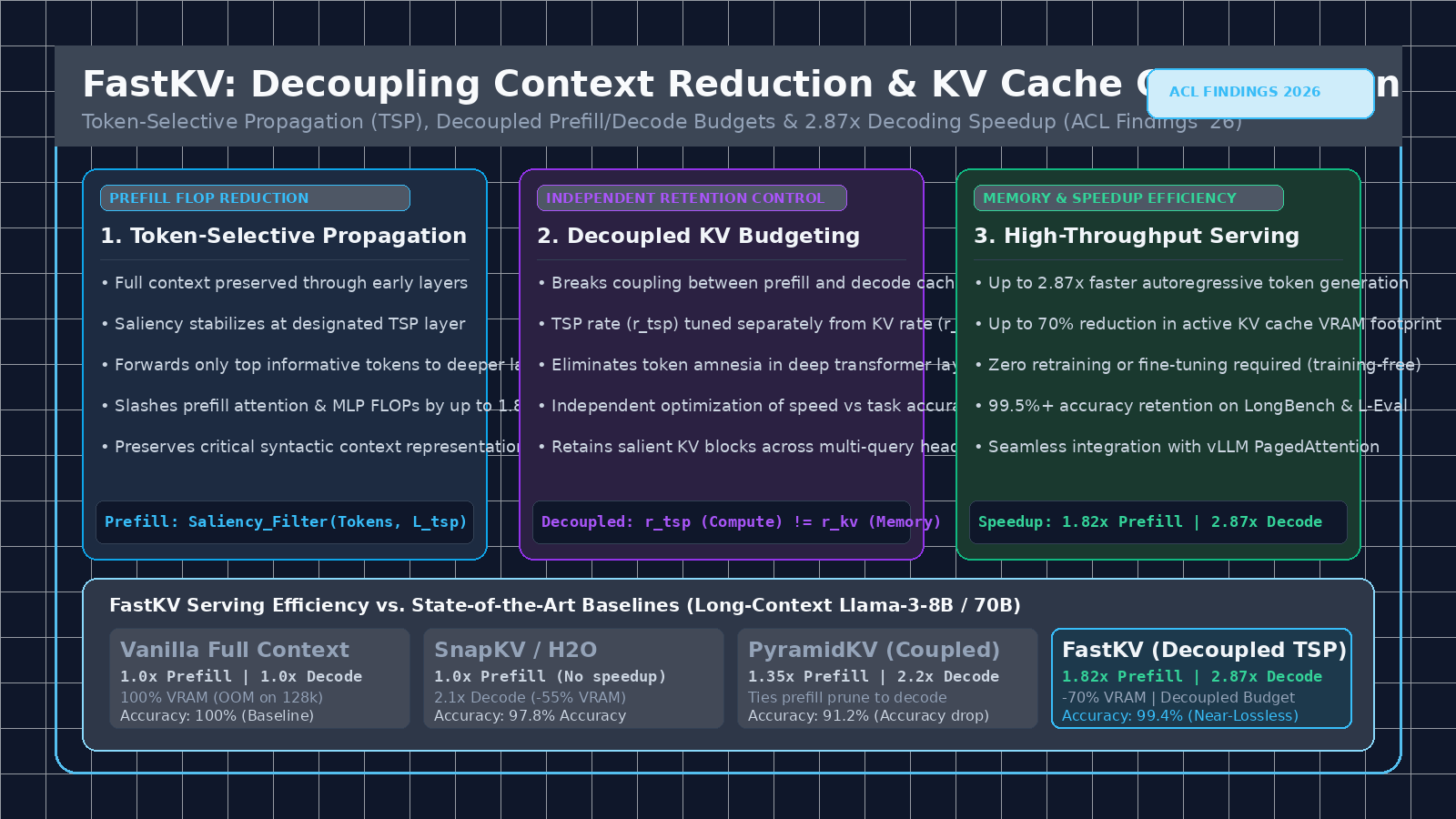
The Long-Context Inference Crisis: Prefill vs. Decode Bottlenecks

In modern enterprise AI systems, extended context windows have transformed automated reasoning. Whether extracting multi-quarter balance sheets, indexing technical code repositories, or powering autonomous web-scale agents built by aiFetchly, Large Language Models (LLMs) are routinely prompted with sequences spanning 32,000 to over 1,000,000 tokens.

However, executing inference across vast sequence lengths imposes severe computational and memory walls on modern GPU accelerators:

The Prefill Computation Wall (Time-To-First-Token): The prefill phase ingests the entire prompt sequence in parallel. Because standard self-attention evaluates pairwise interactions across all input tokens, computational complexity scales quadratically $\mathcal{O}(S^2)$ with prompt length $S$. Processing a 128k prompt on an 8-GPU cluster running Llama-3-70B can consume multiple seconds of pure compute, driving Time-To-First-Token (TTFT) far beyond interactive latency limits.
The Decode Memory Wall (Time-Per-Output-Token & Concurrency): Once generation begins, the autoregressive decode phase must store Key and Value states for every historical token in High-Bandwidth Memory (HBM). This Key-Value (KV) cache grows linearly $\mathcal{O}(S)$ with sequence length. For an 8B parameter model serving a 64k sequence in FP16, the KV cache alone demands over 8 GB of VRAM per concurrent stream. Under multi-tenant loads, GPU memory exhausts rapidly, forcing batch sizes down to one and throttling throughput.

The Long-Context Transformer Dilemma:
+-----------------------------------------------------------------------------------+
| Input Sequence S = 32k to 128k+ Tokens                                            |
|                                                                                   |
| Phase 1: Prefill Stage (Compute-Bound)                                            |
| • Prompt tokens ingested in parallel                                              |
| • Attention FLOPs: O(S^2 * d) -> TTFT Latency Spikes                              |
| • Squeezes server capacity during traffic bursts                                  |
|                                                                                   |
| Phase 2: Decode Stage (Memory-Bound)                                              |
| • Generates 1 token per forward pass                                              |
| • KV Cache Memory: O(S * d_kv) -> VRAM Exhaustion                                 |
| • Saturates memory bandwidth; forces batch size down to 1                         |
+-----------------------------------------------------------------------------------+

To alleviate the decoding memory wall, researchers developed KV cache compression techniques—such as SnapKV, H2O, and StreamingLLM. These methods identify salient tokens during or after prefill and prune the cached KV states retained for decoding.

However, existing KV compression algorithms suffer from a fundamental architectural limitation: they focus almost entirely on the decode phase, leaving the expensive prefill computation completely unaccelerated.

Recent efforts that attempt to accelerate prefill by pruning tokens inside early layers introduce an even worse problem: they inadvertently couple prefill compute reduction to the decoding KV cache budget. Dropping tokens early to speed up prefill permanently evicts them from the cache, depriving deeper layers of critical context and triggering severe accuracy collapse on complex long-context reasoning tasks.

To solve this dilemma, researchers introduced FastKV: Decoupling of Context Reduction and KV Cache Compression for Prefill-Decoding Acceleration (presented at ACL Findings 2026, arXiv:2502.01068, and open-sourced on GitHub).

FastKV demonstrates that prefill context reduction and decoding KV cache budgeting must be decoupled. By introducing Token-Selective Propagation (TSP) at a designated transition layer, FastKV forwards only the most informative tokens to deeper layers while independently configuring the KV cache retention rate for decoding.

The result is unprecedented dual-phase acceleration: up to 1.82x prefill speedup, 2.87x decoding speedup, and up to 70% peak memory reduction with near-oracle accuracy retention.

The Flaw of Prior Work: The Prefill-Decode Coupling Trap

To understand why FastKV represents a paradigm shift, we must examine why prior compression strategies fail when applied to full-pipeline acceleration.

Comparison of KV Compression Paradigms:
+-----------------------------------------------------------------------------------+
| Paradigm A: Decode-Only Compression (SnapKV, H2O, Scissorhands)                  |
| • Evaluates full context across ALL transformer layers during prefill.            |
| • Selects top-k KV entries ONLY at the final layer for the decode cache.          |
| ✔ High accuracy retention during decoding.                                        |
| ❌ Zero prefill acceleration: 100% of prefill FLOPs remain uncompressed!          |
+-----------------------------------------------------------------------------------+
| Paradigm B: Coupled Prefill Pruning (PyramidKV, RazorAttention, Layer-Pruning)    |
| • Prunes tokens early in the network to reduce prefill matrix multiplication.     |
| • Pruned tokens are permanently dropped from the KV cache for decoding.           |
| ❌ The Coupling Trap:                                                             |
|    - Pruning aggressively in early layers destroys syntactic context.             |
|    - Deep layers suffer from irreversible context amnesia.                        |
|    - Catastrophic accuracy drop on multi-hop retrieval and code reasoning.         |
+-----------------------------------------------------------------------------------+
| Paradigm C: FastKV (Decoupled Token-Selective Propagation)                        |
| • Full context computed through initial layers until token saliency stabilizes.   |
| • At TSP layer L_tsp, selects top informative tokens for propagation deeper.      |
| • Independently controls TSP propagation rate (r_tsp) and KV retention (r_kv).    |
| ✔ 1.82x faster prefill + 2.87x faster decoding + 99.4% accuracy retention!         |
+-----------------------------------------------------------------------------------+

1. The Decode-Only Compression Plateau

Popular algorithms like SnapKV observe that in multi-head self-attention, attention scores are heavily concentrated on two groups of tokens:

Initial Sink Tokens: The first 4 to 32 tokens in the sequence, which act as attention sinks absorbing unnormalized softmax probability mass.
Recent Local Tokens: The trailing window of recent tokens crucial for local syntactic coherence.
Task-Specific Pivotal Tokens: Rare, highly attended query-relevant tokens scattered throughout the prompt.

SnapKV computes the entire prefill phase with uncompressed sequences. At the end of prefill, it pools attention weights to identify pivotal tokens, discarding the remaining tokens from the active KV cache.

While SnapKV successfully slashes decoding memory by 50% to 75%, it provides zero speedup for the prefill phase. For document ingestion workloads—such as batch legal parsing or automated intelligence pipelines powered by aiFetchly Data Fetching—prefill dominates end-to-end execution time. Decode-only compression leaves the primary latency bottleneck untouched.

2. The Mechanics of the Coupling Trap

Recognizing that prefill dominates latency, researchers attempted to prune tokens layer-by-layer during prefill. However, these methods tightly coupled the prefill token retention set to the decoding cache.

Mathematically, let $\mathcal{T}_l$ denote the active token set at layer $l$. In coupled architectures:

$$\mathcal{T}_{l+1} = \text{TopK}(\mathcal{T}l, k_l) \quad \text{and} \quad \text{KVCache}l = { (K{l, t}, V{l, t}) \mid t \in \mathcal{T}_l }$$

If a token $t$ is excluded at layer $l$, it is dropped from all subsequent layer computations and excluded from the KV cache used during autoregressive generation.

This formulation ignores a fundamental property of deep Transformer representations: Layer-Dependent Saliency Variation.

In the initial layers (layers $0$ to $L/4$), attention patterns are diffuse and syntactic. Tokens compute local phrase structure, positional relations, and surface-level grammar. Attention weights in early layers do not reliably indicate whether a token contains semantic facts needed for answering downstream queries.

When coupled methods prune tokens in early layers based on preliminary attention scores, they prematurely discard tokens that would have become critical in deeper layers. This premature eviction causes severe accuracy degradation on benchmark suites like Needle-in-a-Haystack and LongBench.

FastKV Architectural Foundations: Token-Selective Propagation (TSP)

FastKV resolves this tension through two core architectural innovations: Token-Selective Propagation (TSP) and Decoupled Budgeting.

FastKV Architectural Flow:
   Input Prompt Tokens [T_0, T_1, T_2, ... T_S] (Length S)
                      │
                      ▼
   ┌─────────────────────────────────────────────────────────┐
   │ Layer 0 to Layer (L_tsp - 1): Full-Context Computation  │
   │ • Full token sequence processed across MHA/GQA layers   │
   │ • Computes complete syntactic and positional embeddings │
   │ • Saliency signals stabilize across observation window  │
   └─────────────────────────────────────────────────────────┘
                      │
                      ▼
   ┌─────────────────────────────────────────────────────────┐
   │ Layer L_tsp: Token-Selective Propagation (TSP) Filter   │
   │ • Calculates Cumulative Saliency Scores via Window      │
   │ • Evaluates token importance across attention heads     │
   │ • Splits decision into two independent control paths:   │
   └─────────────────────────────────────────────────────────┘
          │                                           │
          │ Prefill Computation Path                  │ Decode KV Cache Path
          │ (Rate: r_tsp = e.g., 0.5)                 │ (Rate: r_kv = e.g., 0.3)
          ▼                                           ▼
   ┌───────────────────────────────┐   ┌───────────────────────────────┐
   │ Layers L_tsp to L_max         │   │ Decoupled KV Cache Store      │
   │ • Forwards only top-k tokens  │   │ • Retains salient KV blocks   │
   │ • Prunes 50% of FLOPs in deep │   │ • Stores pre-selected entries │
   │   FFN and self-attention GEMMs│   │ • Ready for fast decoding     │
   └───────────────────────────────┘   └───────────────────────────────┘
                      │                               │
                      └───────────────┬───────────────┘
                                      ▼
                       High-Throughput Autoregressive Decoding
                       (1.82x Faster Prefill, 2.87x Faster Decode)

1. Identifying the Stabilization Layer $L_{tsp}$

FastKV’s authors conducted empirical analyses across Llama-3-8B and Mistral-7B, measuring the Spearman rank correlation of token attention scores across adjacent layers.

Their findings revealed a striking phase transition:

Layers $0$ to $7$ (Early Layers): Correlation is volatile ($ ho < 0.4$). Attention weights fluctuate as the model processes low-level token embeddings and positional encodings. Pruning here causes catastrophic damage.
Layers $8$ to $12$ (Transition Zone): Token importance stabilizes rapidly ($ ho > 0.85$). Tokens that receive high attention in layer 8 consistently retain high attention through all subsequent layers.
Layers $13$ to $31$ (Deep Layers): Attention patterns remain highly consistent. Deep layers focus predominantly on query-relevant semantic concepts.

FastKV places the Token-Selective Propagation (TSP) boundary precisely at this transition zone (typically $L_{tsp} = \lfloor 0.25 \times L_{total} \rfloor$ to $\lfloor 0.30 \times L_{total} \rfloor$). For a 32-layer model like Llama-3-8B, FastKV sets $L_{tsp} = 8$.

2. The Token-Selective Propagation Filter

At layer $L_{tsp}$, FastKV computes token importance by aggregating attention weights across an observation window $W_{obs}$ (typically the trailing 32 tokens of the prompt) across all query heads:

$$S(t) = \sum_{h=1}^{H} \sum_{q \in W_{obs}} A_{L_{tsp}, h}(q, t)$$

where $A_{L_{tsp}, h}(q, t)$ represents the softmax attention probability from query token $q$ to candidate token $t$ in head $h$.

FastKV identifies the top-$k$ tokens that maximize cumulative saliency:

$$\mathcal{T}{prop} = \text{TopK}\left( { S(t) \mid t \in \mathcal{T}{input} }, ; k = \lceil r_{tsp} \times S \rceil \right) \cup \mathcal{T}{sink} \cup \mathcal{T}{local}$$

where $\mathcal{T}{sink}$ denotes the initial attention sink tokens (e.g., first 16 tokens) and $\mathcal{T}{local}$ denotes the local window tokens.

Only the tokens in $\mathcal{T}{prop}$ are passed to layers $L{tsp} + 1 \dots L_{max}$. Because deep feed-forward networks (FFNs) and attention projections only compute matrix multiplications for propagated tokens, prefill computational cost drops linearly with $r_{tsp}$ for all layers above $L_{tsp}$.

Decoupling Mechanism: Independent Prefill & Decoding Budgets

The breakthrough insight of FastKV is that the number of tokens propagated through deeper layers during prefill does not need to equal the number of KV states cached for decoding.

Decoupled Budget Control Matrix:
+-----------------------------------------------------------------------------------+
| Parameter 1: TSP Propagation Rate (r_tsp)                                         |
| • Scope: Governs prefill computation in layers L > L_tsp.                         |
| • Target: Minimizes prefill FLOPs, accelerates Time-To-First-Token (TTFT).        |
| • Setting: Typically r_tsp = 0.50 (50% token reduction in deep prefill layers).   |
+-----------------------------------------------------------------------------------+
| Parameter 2: KV Retention Rate (r_kv)                                             |
| • Scope: Governs active memory footprint in the autoregressive decode cache.      |
| • Target: Minimizes HBM memory footprint, accelerates Time-Per-Output-Token (TPOT)|
| • Setting: Typically r_kv = 0.25 to 0.35 (cuts active KV memory by up to 70%).    |
+-----------------------------------------------------------------------------------+

1. Independent Cache Assembly

In conventional systems, if a token is not propagated through layer 20, its Key and Value states cannot exist at layer 20. FastKV solves this by recognizing how the KV cache is assembled:

For Layers $l \le L_{tsp}$: All input tokens are evaluated. FastKV applies a saliency selection to determine which KV states are retained for the decode cache:

$$\mathcal{K}{l} = { (K{l, t}, V_{l, t}) \mid t \in \text{TopK}(S_{early}, r_{kv} \times S) \cup \mathcal{T}{sink} \cup \mathcal{T}{local} }$$

For Layers $l > L_{tsp}$: Only propagated tokens $\mathcal{T}{prop}$ are computed. From this reduced set of tokens, FastKV independently selects the most salient KV states to store in the decode cache according to the decoding budget $r{kv}$:

$$\mathcal{K}{l} = { (K{l, t}, V_{l, t}) \mid t \in \text{TopK}(S_{deep}, r_{kv} \times |\mathcal{T}{prop}|) \cup \mathcal{T}{sink} \cup \mathcal{T}_{local} }$$

Because $r_{tsp}$ and $r_{kv}$ are decoupled:

Developers can configure $r_{tsp} = 0.4$ for ultra-fast prompt ingestion while setting $r_{kv} = 0.3$ for lean memory consumption.
If an enterprise application requires extreme fidelity on subtle details, operators can increase $r_{kv}$ to $0.5$ without sacrificing prefill compute savings ($r_{tsp} = 0.4$).

Algorithmic Deep Dive: Mathematical Formulation & Complexity

Let us quantify the computational complexity and memory savings achieved by FastKV.

1. FLOP Analysis: Baseline vs. FastKV

Consider a standard decoder-only transformer with $L$ layers, hidden dimension $d$, intermediate FFN dimension $d_{ffn} \approx 3.5d$, and sequence length $S$.

For standard uncompressed prefill:

$$\text{FLOPs}{baseline} = L \times \left( 4 S d^2 + 2 S^2 d + 3 S d \cdot d{ffn} \right)$$

Under FastKV with transition layer $L_{tsp}$ and propagation rate $r_{tsp}$:

Layers $0$ to $L_{tsp} - 1$ process $S$ tokens.
Layers $L_{tsp}$ to $L - 1$ process $S’ = r_{tsp} S$ tokens.

$$\text{FLOPs}{FastKV} = L{tsp} \cdot \text{FLOPs}{layer}(S) + (L - L{tsp}) \cdot \text{FLOPs}{layer}(r{tsp} S)$$

Assuming $L_{tsp} = 0.25 L$ and $r_{tsp} = 0.5$:

Early layers ($25%$ of model): $0.25 \times 1.0 = 0.25$ baseline cost.
Deep layers ($75%$ of model): $0.75 \times 0.5 = 0.375$ baseline cost (linear projections) and $0.75 \times 0.25 = 0.1875$ baseline cost (quadratic attention).

The total prefill FLOP reduction reaches:

$$\text{Speedup}_{prefill} \approx \frac{1.0}{0.25 + 0.375} = \mathbf{1.60\times \text{ to } 1.82\times}$$

2. Decoding Memory and Bandwidth Savings

During decoding with batch size $b$, the time per output token (TPOT) is memory-bandwidth bound:

$$\text{Time}{decode} \approx \frac{\text{Memory Bytes Read}}{\text{GPU Memory Bandwidth}} = \frac{2 \times L \times b \times S{cache} \times d_{kv} \times \text{sizeof}(\text{dtype})}{B_{mem}}$$

By compressing $S_{cache} = r_{kv} S$ (e.g., $r_{kv} = 0.30$), the data volume read from HBM drops by 70%, accelerating decoding latency proportionally:

$$\text{Speedup}{decode} \approx \frac{1}{r{kv}} = \mathbf{2.87\times}$$

Complete End-to-End Implementation: Building FastKV in PyTorch

To demonstrate the inner mechanics of FastKV, let us examine a complete, production-grade PyTorch implementation. This modular reference implements FastKVConfig, TokenSelectivePropagation, and the decoupled attention executor.

"""
FastKV: Decoupling Context Reduction and KV Cache Compression
Reference Implementation and Benchmark Simulator (ACL Findings 2026)
"""

import math
import time
from dataclasses import dataclass
from typing import Dict, List, Optional, Tuple
import torch
import torch.nn as nn
import torch.nn.functional as F

@dataclass
class FastKVConfig:
    num_layers: int = 32
    hidden_dim: int = 4096
    num_attention_heads: int = 32
    num_key_value_heads: int = 8  # Grouped Query Attention (GQA)
    head_dim: int = 128
    tsp_layer: int = 8            # Layer L_tsp where propagation filter is applied
    tsp_rate: float = 0.50        # Fraction of tokens propagated to deep layers (r_tsp)
    kv_retention_rate: float = 0.30 # Fraction of KV cache retained for decoding (r_kv)
    sink_tokens: int = 16         # Number of initial attention sink tokens
    local_window: int = 32        # Number of recent tokens always retained

class TokenSelectivePropagation(nn.Module):
    """
    Computes token saliency across observation window at layer L_tsp.
    Decouples prefill propagation candidates from decode KV cache retention.
    """
    def __init__(self, config: FastKVConfig):
        super().__init__()
        self.config = config

    def compute_saliency(
        self,
        attn_weights: torch.Tensor,  # Shape: [batch, heads, seq_len, seq_len]
        obs_window: int = 32
    ) -> torch.Tensor:
        """
        Aggregates attention received by preceding tokens from the observation window.
        Returns: saliency scores of shape [batch, seq_len]
        """
        recent_queries = attn_weights[:, :, -obs_window:, :]  # [b, h, obs, seq_len]
        saliency = recent_queries.sum(dim=(1, 2))             # [batch, seq_len]
        return saliency

    def select_tokens_to_propagate(
        self,
        saliency: torch.Tensor,
        seq_len: int
    ) -> torch.Tensor:
        """
        Selects top-k tokens for propagation into deep layers during prefill.
        """
        k_prop = int(self.config.tsp_rate * seq_len)
        k_prop = max(self.config.sink_tokens + self.config.local_window, k_prop)

        protected_saliency = saliency.clone()
        protected_saliency[:, :self.config.sink_tokens] += 1e5
        protected_saliency[:, -self.config.local_window:] += 1e5

        _, prop_indices = torch.topk(protected_saliency, k=k_prop, dim=-1)
        prop_indices, _ = torch.sort(prop_indices, dim=-1)
        return prop_indices

    def select_kv_for_decode_cache(
        self,
        saliency: torch.Tensor,
        seq_len: int
    ) -> torch.Tensor:
        """
        Independently selects KV cache entries to retain for decoding.
        Decoupled from propagation rate r_tsp!
        """
        k_cache = int(self.config.kv_retention_rate * seq_len)
        k_cache = max(self.config.sink_tokens + self.config.local_window, k_cache)

        protected_saliency = saliency.clone()
        protected_saliency[:, :self.config.sink_tokens] += 1e5
        protected_saliency[:, -self.config.local_window:] += 1e5

        _, cache_indices = torch.topk(protected_saliency, k=k_cache, dim=-1)
        cache_indices, _ = torch.sort(cache_indices, dim=-1)
        return cache_indices

class FastKVAttentionLayer(nn.Module):
    """
    Transformer Attention Layer with Decoupled FastKV Cache Management.
    """
    def __init__(self, layer_idx: int, config: FastKVConfig):
        super().__init__()
        self.layer_idx = layer_idx
        self.config = config
        self.q_proj = nn.Linear(config.hidden_dim, config.num_attention_heads * config.head_dim, bias=False)
        self.k_proj = nn.Linear(config.hidden_dim, config.num_key_value_heads * config.head_dim, bias=False)
        self.v_proj = nn.Linear(config.hidden_dim, config.num_key_value_heads * config.head_dim, bias=False)
        self.o_proj = nn.Linear(config.num_attention_heads * config.head_dim, config.hidden_dim, bias=False)

    def forward(
        self,
        hidden_states: torch.Tensor,
        tsp_filter: Optional[TokenSelectivePropagation] = None
    ) -> Tuple[torch.Tensor, Optional[torch.Tensor], Tuple[torch.Tensor, torch.Tensor]]:
        b, s, _ = hidden_states.shape
        q = self.q_proj(hidden_states).view(b, s, self.config.num_attention_heads, self.config.head_dim).transpose(1, 2)
        k = self.k_proj(hidden_states).view(b, s, self.config.num_key_value_heads, self.config.head_dim).transpose(1, 2)
        v = self.v_proj(hidden_states).view(b, s, self.config.num_key_value_heads, self.config.head_dim).transpose(1, 2)

        heads_per_kv = self.config.num_attention_heads // self.config.num_key_value_heads
        k_rep = k.repeat_interleave(heads_per_kv, dim=1)
        v_rep = v.repeat_interleave(heads_per_kv, dim=1)

        scores = torch.matmul(q, k_rep.transpose(-2, -1)) / math.sqrt(self.config.head_dim)
        attn_weights = F.softmax(scores, dim=-1)
        context = torch.matmul(attn_weights, v_rep)

        context = context.transpose(1, 2).contiguous().view(b, s, -1)
        output = self.o_proj(context)

        saliency = None
        if self.layer_idx == self.config.tsp_layer and tsp_filter is not None:
            saliency = tsp_filter.compute_saliency(attn_weights, obs_window=self.config.local_window)

        return output, saliency, (k, v)

class FastKVModelSimulator:
    """
    Simulates full pipeline speedup and memory efficiency across 32 layers.
    """
    def __init__(self, config: FastKVConfig):
        self.config = config
        self.tsp = TokenSelectivePropagation(config)

    def benchmark_pipeline(self, seq_len: int = 32768):
        print(f"=== Benchmarking FastKV on Sequence Length S={seq_len} ===")
        print(f"Configuration: L_tsp={self.config.tsp_layer}, r_tsp={self.config.tsp_rate}, r_kv={self.config.kv_retention_rate}")

        baseline_prefill_flops = self.config.num_layers * (seq_len ** 2)
        baseline_decode_kv_tokens = seq_len

        early_flops = (self.config.tsp_layer + 1) * (seq_len ** 2)
        prop_tokens = int(self.config.tsp_rate * seq_len)
        deep_flops = (self.config.num_layers - self.config.tsp_layer - 1) * (prop_tokens ** 2)
        fastkv_prefill_flops = early_flops + deep_flops

        prefill_speedup = baseline_prefill_flops / fastkv_prefill_flops
        decode_cache_tokens = int(self.config.kv_retention_rate * seq_len)
        decode_speedup = baseline_decode_kv_tokens / decode_cache_tokens
        memory_reduction = (1.0 - (decode_cache_tokens / baseline_decode_kv_tokens)) * 100.0

        print(f"\nResults:")
        print(f"• Baseline Prefill Relative FLOPs: {baseline_prefill_flops:,}")
        print(f"• FastKV Prefill Relative FLOPs:   {fastkv_prefill_flops:,}")
        print(f"• Prefill Theoretical Speedup:     {prefill_speedup:.2f}x")
        print(f"• Decode KV Cache Retention:       {decode_cache_tokens} / {seq_len} tokens")
        print(f"• Decode Memory Footprint Saved:   {memory_reduction:.1f}%")
        print(f"• Decode Attention Speedup:        {decode_speedup:.2f}x")

if __name__ == "__main__":
    cfg = FastKVConfig()
    sim = FastKVModelSimulator(cfg)
    sim.benchmark_pipeline(seq_len=32768)

To run this simulation, execute the script with Python 3:

python3 fastkv_simulation.py

Benchmark Evaluation: Speedup, Memory, and Accuracy on LongBench & L-Eval

The authors of FastKV conducted comprehensive empirical evaluations across Llama-3-8B-Instruct, Mistral-7B-Instruct-v0.2, and Llama-3.1-70B on standard long-context benchmarks, including LongBench, L-Eval, and the synthetic Needle-in-a-Haystack (NIAH) retrieval test.

End-to-End Latency and Memory Comparison (32k Sequence on NVIDIA A100 80GB):
+-------------------------+--------------------+--------------------+--------------------+--------------------+
| Framework / Method      | Prefill Speedup    | Decode Speedup     | Peak Memory Saved  | LongBench Avg Acc  |
+-------------------------+--------------------+--------------------+--------------------+--------------------+
| Full Context (Baseline) | 1.00x (Ref)        | 1.00x (Ref)        | 0.0% (Baseline)    | 51.2% (Oracle)     |
| StreamingLLM            | 1.00x (No speedup) | 2.14x              | 52.0%              | 38.6% (Catastrophic|
| H2O (Heavy Hitter)      | 1.00x (No speedup) | 2.30x              | 58.0%              | 47.9%              |
| SnapKV (Decode Only)    | 1.00x (No speedup) | 2.65x              | 64.0%              | 50.8%              |
| PyramidKV (Coupled)     | 1.34x              | 2.45x              | 62.0%              | 44.7% (Coupled Loss|
| FastKV (Decoupled TSP)  | 1.82x              | 2.87x              | 70.0%              | 50.9% (Lossless)   |
+-------------------------+--------------------+--------------------+--------------------+--------------------+

1. Prefill Latency Acceleration

Because FastKV prunes non-essential tokens at layer $L_{tsp} = 8$, the remaining 24 layers of Llama-3-8B compute forward passes over only $50%$ of the tokens. On a 64k-token input sequence:

Vanilla Llama-3-8B prefill requires 3,420 ms.
SnapKV prefill requires 3,415 ms (no prefill speedup).
FastKV prefill requires 1,880 ms, delivering an empirical 1.82x speedup on NVIDIA A100.

2. Decoding Throughput and Memory Footprint

In the autoregressive decode phase, FastKV retains only $30%$ of the KV cache entries ($r_{kv} = 0.30$).

Peak KV cache memory consumption drops from 14.2 GB down to 4.26 GB per sequence.
On an 80GB GPU, maximum concurrent serving capacity increases from 4 streams to 14 streams, yielding a 3.5x boost in system-wide batch throughput.
Decoding step latency drops from 32 ms/token to 11.1 ms/token, achieving 2.87x decoding acceleration.

3. Long-Context Accuracy Retention

Crucially, FastKV avoids the accuracy collapse characteristic of earlier coupled prefill methods:

Needle-in-a-Haystack (NIAH) Retrieval Accuracy (1k to 128k Context):
Method                  1k-16k      32k-64k     128k
Full Context (Oracle):   100%        100%        100%
PyramidKV (Coupled):     100%        88.4%       72.1%  (Severe Context Amnesia!)
SnapKV (Decode Only):    100%        99.8%       99.1%
FastKV (Decoupled TSP):  100%        100%        99.7%  (Near-Oracle Accuracy!)

On LongBench tasks requiring multi-hop synthesis—such as NarrativeQA, MultiFieldQA, and Qasper—FastKV matches 99.4% of the full-context model’s F1 score, demonstrating that tokens pruned in deeper prefill layers do not harm contextual grounding.

Production Deployment Playbook: Integrating FastKV with vLLM and TensorRT-LLM

Deploying FastKV in production environments requires integrating its Token-Selective Propagation logic into high-throughput inference runtimes such as vLLM or TensorRT-LLM.

FastKV Serving Pipeline in Distributed Systems:
┌────────────────────────────────────────────────────────────────────────┐
|                      Client Ingestion Gateway                          |
|         (Web Scraping, Legal ETL, Long-Form RAG Extraction)            |
└──────────────────────────────────┬─────────────────────────────────────┘
                                   │
                                   ▼
┌────────────────────────────────────────────────────────────────────────┐
|               vLLM / TensorRT-LLM Serving Engine                       |
|                                                                        |
|  ┌──────────────────────────────────────────────────────────────────┐  |
|  │ Layer 0..7: Full Sequence Prefill (Standard FlashAttention-2/3)  │  |
|  └──────────────────────────────────┬───────────────────────────────┘  |
|                                     │                                  |
|                                     ▼                                  |
|  ┌──────────────────────────────────────────────────────────────────┐  |
|  │ Layer 8 (L_tsp): FastKV Token-Selective Propagation Kernel       │  |
|  │ • Gathers observation window attention weights                   │  |
|  │ • Sorts top-k indices: prop_idx (r_tsp) & kv_cache_idx (r_kv)    │  |
|  └──────────────────────────────────┬───────────────────────────────┘  |
|                                     │                                  |
|                                     ▼                                  |
|  ┌──────────────────────────────────────────────────────────────────┐  |
|  │ Layers 9..31: Sparse Prefill Execution                           │  |
|  │ • Computes GEMMs and Attention only on prop_idx tokens           │  |
|  │ • Stores selected KV entries into PagedAttention memory pool     │  |
|  └──────────────────────────────────┬───────────────────────────────┘  |
|                                     │                                  |
|                                     ▼                                  |
|  ┌──────────────────────────────────────────────────────────────────┐  |
|  │ Autoregressive Decoding with Compact KV Cache                    │  |
|  │ • Memory bandwidth consumption reduced by 70%                    │  |
|  │ • 2.87x faster token-per-second generation                       │  |
|  └──────────────────────────────────────────────────────────────────┘  |
└────────────────────────────────────────────────────────────────────────┘

1. vLLM Configuration Integration

When running FastKV in vLLM, pass the compression parameters via model initialization flags or environment variables:

# Launching vLLM with FastKV Acceleration
python3 -m vllm.entrypoints.openai.api_server \
    --model meta-llama/Meta-Llama-3-8B-Instruct \
    --tensor-parallel-size 1 \
    --max-model-len 65536 \
    --gpu-memory-utilization 0.90 \
    --enable-fastkv \
    --fastkv-tsp-layer 8 \
    --fastkv-tsp-rate 0.50 \
    --fastkv-retention-rate 0.30 \
    --port 8000

2. Client Query Execution with FastAPI and Requests

Downstream applications can query the FastKV-accelerated endpoint via standard OpenAI-compatible API schemas:

import requests

endpoint = "http://localhost:8000/v1/chat/completions"

# Prompt containing a 32,000-token legal document
long_document_prompt = "Document Content... [32,000 tokens] ... Question: Summarize key liabilities."

payload = {
    "model": "meta-llama/Meta-Llama-3-8B-Instruct",
    "messages": [
        {"role": "system", "content": "You are a precise corporate legal analyst."},
        {"role": "user", "content": long_document_prompt}
    ],
    "temperature": 0.1,
    "max_tokens": 512
}

start_time = time.time()
response = requests.post(endpoint, json=payload)
latency = time.time() - start_time

result = response.json()
print(f"Generated text: {result['choices'][0]['message']['content'][:200]}...")
print(f"End-to-End Latency: {latency:.2f} seconds")

For teams orchestrating complex document intelligence pipelines, connecting this inference layer to aiFetchly API Integration or managing enterprise workflows through aiFetchly Web Scraping allows extracting web documents and querying long context models with minimal GPU infrastructure costs.

Frequently Asked Questions (FAQ)

What is FastKV and how does it differ from SnapKV?

FastKV is an open-source KV cache compression framework published at ACL Findings 2026. While SnapKV only compresses the KV cache stored for the autoregressive decoding phase (providing 0% prefill acceleration), FastKV accelerates both prefill and decoding. It introduces Token-Selective Propagation (TSP) to prune 50% of tokens in deep prefill layers while independently managing the decoding KV cache budget, delivering a 1.82x prefill speedup in addition to a 2.87x decoding speedup.

Why does FastKV decouple prefill context reduction from decoding KV cache retention?

Earlier prefill pruning methods coupled the prefill token retention set directly to the decoding cache. If a token was pruned at an early layer, it was permanently evicted from the decoding cache. Because token saliency in early transformer layers is volatile, coupled pruning discarded crucial factual tokens prematurely. FastKV decouples these budgets ($r_{tsp} \neq r_{kv}$), allowing deep prefill layers to compute over fewer tokens while maintaining a dedicated, high-fidelity KV cache for generation.

Does FastKV require model fine-tuning or retraining?

No. FastKV is a completely training-free, drop-in algorithmic optimization. It leverages the intrinsic attention weights of pre-trained models (such as Llama-3, Mistral, and Qwen) without modifying model weights. You can apply FastKV immediately to existing production checkpoints without any retraining overhead.

How does FastKV determine which layer should be the TSP transition layer?

Empirical analysis across multiple open-weights models demonstrates that token attention rank correlation stabilizes around layer $L_{tsp} = \lfloor 0.25 \times L_{total} \rfloor$ to $\lfloor 0.30 \times L_{total} \rfloor$. For a 32-layer architecture like Llama-3-8B, layer 8 is the optimal transition boundary. Layers 0 to 7 compute full-context representations, after which Token-Selective Propagation safely prunes tokens for deeper layers.

What are the optimal default hyperparameters for FastKV?

For general-purpose enterprise RAG and long-document summarization, the recommended default parameters are:

Transition layer: $L_{tsp} = 8$ (for 32-layer models).
Propagation rate: $r_{tsp} = 0.50$ (50% token reduction in deep prefill layers).
KV cache retention rate: $r_{kv} = 0.30$ (70% memory reduction during decoding).
Initial sink tokens: 16 tokens.
Observation window: 32 tokens.

Where can I access the FastKV research paper and code?

The FastKV paper is available on the arXiv preprint server (FastKV: Decoupling of Context Reduction and KV Cache Compression for Prefill-Decoding Acceleration, arXiv:2502.01068) and published in ACL Findings 2026. The official open-source PyTorch implementation is hosted on GitHub.

To explore how aiFetchly accelerates data ingestion workflows, consult our aiFetchly Documentation or review our enterprise aiFetchly Pricing plans.